Repository of Reproducible Computations

Free Statistics

of Irreproducible Research!

Author's title

Author

*Unverified author*

R Software Module

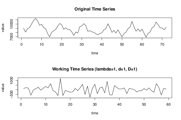
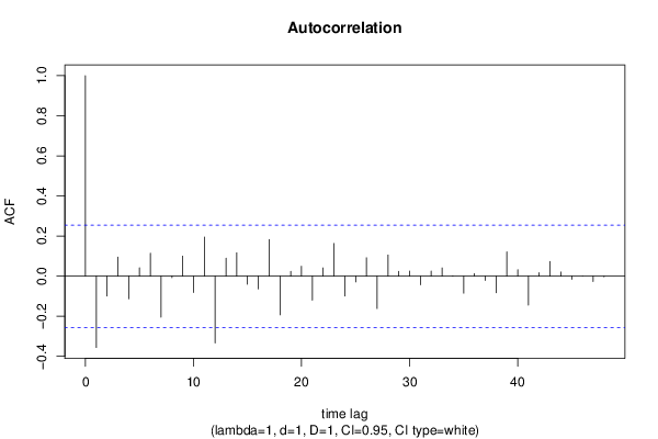
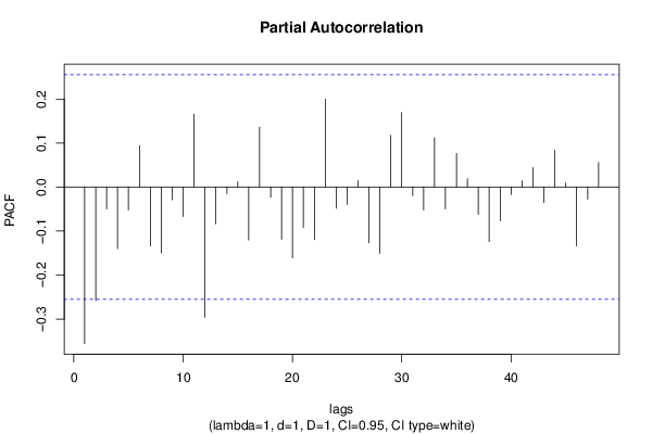
Title produced by software

(Partial) Autocorrelation Function

Date of computation

Tue, 04 Dec 2012 11:47:10 -0500

Cite this page as follows

Statistical Computations at FreeStatistics.org, Office for Research Development and Education, URL https://freestatistics.org/blog/index.php?v=date/2012/Dec/04/t1354639651qpssox0d1yj0pg0.htm/, Retrieved Tue, 16 Apr 2024 17:50:34 +0000

Statistical Computations at FreeStatistics.org, Office for Research Development and Education, URL https://freestatistics.org/blog/index.php?pk=196385, Retrieved Tue, 16 Apr 2024 17:50:34 +0000

QR Codes:

Paste this QR Code to cite your computation.

Original text written by user:

IsPrivate?

No (this computation is public)

User-defined keywords

Estimated Impact

Family? (F = Feedback message, R = changed R code, M = changed R Module, P = changed Parameters, D = changed Data)

-     [Univariate Explorative Data Analysis] [Run Sequence gebo...] [2008-12-12 13:32:37] [76963dc1903f0f612b6153510a3818cf]
- R  D  [Univariate Explorative Data Analysis] [Run Sequence gebo...] [2008-12-17 12:14:40] [76963dc1903f0f612b6153510a3818cf]
-         [Univariate Explorative Data Analysis] [Run Sequence Plot...] [2008-12-22 18:19:51] [1ce0d16c8f4225c977b42c8fa93bc163]
- RMP       [Univariate Data Series] [Identifying Integ...] [2009-11-22 12:08:06] [b98453cac15ba1066b407e146608df68]
- RMPD        [(Partial) Autocorrelation Function] [] [2011-12-05 20:11:33] [bdca8f3e7c3554be8c1291e54f61d441]
- RM              [(Partial) Autocorrelation Function] [WS9, 2] [2012-12-04 16:47:10] [d41d8cd98f00b204e9800998ecf8427e] [Current]

Feedback Forum

Post a new message

Dataseries X:

Download CSV

Histogram

Boxplots

Summary of computational transaction
Raw Input	view raw input (R code)
Raw Output	view raw output of R engine
Computing time	2 seconds
R Server	'Herman Ole Andreas Wold' @ wold.wessa.net

\begin{tabular}{lllllllll}
\hline
Summary of computational transaction \tabularnewline
Raw Input & view raw input (R code)  \tabularnewline
Raw Output & view raw output of R engine  \tabularnewline
Computing time & 2 seconds \tabularnewline
R Server & 'Herman Ole Andreas Wold' @ wold.wessa.net \tabularnewline
\hline
\end{tabular}
%Source: https://freestatistics.org/blog/index.php?pk=196385&T=0

[TABLE]
[ROW][C]Summary of computational transaction[/C][/ROW]
[ROW][C]Raw Input[/C][C]view raw input (R code) [/C][/ROW]
[ROW][C]Raw Output[/C][C]view raw output of R engine [/C][/ROW]
[ROW][C]Computing time[/C][C]2 seconds[/C][/ROW]
[ROW][C]R Server[/C][C]'Herman Ole Andreas Wold' @ wold.wessa.net[/C][/ROW]
[/TABLE]
Source: https://freestatistics.org/blog/index.php?pk=196385&T=0

Globally Unique Identifier (entire table): ba.freestatistics.org/blog/index.php?pk=196385&T=0

As an alternative you can also use a QR Code:

The GUIDs for individual cells are displayed in the table below:

Summary of computational transaction
Raw Input	view raw input (R code)
Raw Output	view raw output of R engine
Computing time	2 seconds
R Server	'Herman Ole Andreas Wold' @ wold.wessa.net

Autocorrelation Function
Time lag k	ACF(k)	T-STAT	P-value
1	-0.355844	-2.7333	0.004131
2	-0.098721	-0.7583	0.225648
3	0.09553	0.7338	0.232994
4	-0.112515	-0.8642	0.195476
5	0.041529	0.319	0.37543
6	0.114109	0.8765	0.192161
7	-0.20413	-1.568	0.06112
8	-0.007123	-0.0547	0.478275
9	0.100067	0.7686	0.22259
10	-0.081448	-0.6256	0.26699
11	0.195206	1.4994	0.069551
12	-0.333183	-2.5592	0.006537
13	0.090181	0.6927	0.245609
14	0.116314	0.8934	0.187629
15	-0.040608	-0.3119	0.378103
16	-0.06325	-0.4858	0.314442
17	0.183281	1.4078	0.082218
18	-0.192938	-1.482	0.071833
19	0.024188	0.1858	0.426623
20	0.04958	0.3808	0.352347
21	-0.120146	-0.9229	0.17992
22	0.041112	0.3158	0.376639
23	0.163064	1.2525	0.107662
24	-0.098909	-0.7597	0.22522
25	-0.028902	-0.222	0.412541
26	0.091749	0.7047	0.241873
27	-0.161288	-1.2389	0.110149
28	0.10567	0.8117	0.210122
29	0.02429	0.1866	0.426317
30	0.025905	0.199	0.421481
31	-0.042902	-0.3295	0.371457
32	0.025149	0.1932	0.423744
33	0.04113	0.3159	0.376586
34	0.001673	0.0129	0.494895
35	-0.084857	-0.6518	0.25853
36	0.012637	0.0971	0.4615
37	-0.020799	-0.1598	0.436808
38	-0.082985	-0.6374	0.263159
39	0.121447	0.9329	0.177349
40	0.03188	0.2449	0.403702
41	-0.143982	-1.1059	0.13662
42	0.017224	0.1323	0.4476
43	0.073058	0.5612	0.288404
44	0.020769	0.1595	0.436898
45	-0.01602	-0.1231	0.451242
46	0.000219	0.0017	0.499331
47	-0.026927	-0.2068	0.418429
48	-0.00294	-0.0226	0.491029

\begin{tabular}{lllllllll}
\hline
Autocorrelation Function \tabularnewline
Time lag k & ACF(k) & T-STAT & P-value \tabularnewline
1 & -0.355844 & -2.7333 & 0.004131 \tabularnewline
2 & -0.098721 & -0.7583 & 0.225648 \tabularnewline
3 & 0.09553 & 0.7338 & 0.232994 \tabularnewline
4 & -0.112515 & -0.8642 & 0.195476 \tabularnewline
5 & 0.041529 & 0.319 & 0.37543 \tabularnewline
6 & 0.114109 & 0.8765 & 0.192161 \tabularnewline
7 & -0.20413 & -1.568 & 0.06112 \tabularnewline
8 & -0.007123 & -0.0547 & 0.478275 \tabularnewline
9 & 0.100067 & 0.7686 & 0.22259 \tabularnewline
10 & -0.081448 & -0.6256 & 0.26699 \tabularnewline
11 & 0.195206 & 1.4994 & 0.069551 \tabularnewline
12 & -0.333183 & -2.5592 & 0.006537 \tabularnewline
13 & 0.090181 & 0.6927 & 0.245609 \tabularnewline
14 & 0.116314 & 0.8934 & 0.187629 \tabularnewline
15 & -0.040608 & -0.3119 & 0.378103 \tabularnewline
16 & -0.06325 & -0.4858 & 0.314442 \tabularnewline
17 & 0.183281 & 1.4078 & 0.082218 \tabularnewline
18 & -0.192938 & -1.482 & 0.071833 \tabularnewline
19 & 0.024188 & 0.1858 & 0.426623 \tabularnewline
20 & 0.04958 & 0.3808 & 0.352347 \tabularnewline
21 & -0.120146 & -0.9229 & 0.17992 \tabularnewline
22 & 0.041112 & 0.3158 & 0.376639 \tabularnewline
23 & 0.163064 & 1.2525 & 0.107662 \tabularnewline
24 & -0.098909 & -0.7597 & 0.22522 \tabularnewline
25 & -0.028902 & -0.222 & 0.412541 \tabularnewline
26 & 0.091749 & 0.7047 & 0.241873 \tabularnewline
27 & -0.161288 & -1.2389 & 0.110149 \tabularnewline
28 & 0.10567 & 0.8117 & 0.210122 \tabularnewline
29 & 0.02429 & 0.1866 & 0.426317 \tabularnewline
30 & 0.025905 & 0.199 & 0.421481 \tabularnewline
31 & -0.042902 & -0.3295 & 0.371457 \tabularnewline
32 & 0.025149 & 0.1932 & 0.423744 \tabularnewline
33 & 0.04113 & 0.3159 & 0.376586 \tabularnewline
34 & 0.001673 & 0.0129 & 0.494895 \tabularnewline
35 & -0.084857 & -0.6518 & 0.25853 \tabularnewline
36 & 0.012637 & 0.0971 & 0.4615 \tabularnewline
37 & -0.020799 & -0.1598 & 0.436808 \tabularnewline
38 & -0.082985 & -0.6374 & 0.263159 \tabularnewline
39 & 0.121447 & 0.9329 & 0.177349 \tabularnewline
40 & 0.03188 & 0.2449 & 0.403702 \tabularnewline
41 & -0.143982 & -1.1059 & 0.13662 \tabularnewline
42 & 0.017224 & 0.1323 & 0.4476 \tabularnewline
43 & 0.073058 & 0.5612 & 0.288404 \tabularnewline
44 & 0.020769 & 0.1595 & 0.436898 \tabularnewline
45 & -0.01602 & -0.1231 & 0.451242 \tabularnewline
46 & 0.000219 & 0.0017 & 0.499331 \tabularnewline
47 & -0.026927 & -0.2068 & 0.418429 \tabularnewline
48 & -0.00294 & -0.0226 & 0.491029 \tabularnewline
\hline
\end{tabular}
%Source: https://freestatistics.org/blog/index.php?pk=196385&T=1

[TABLE]
[ROW][C]Autocorrelation Function[/C][/ROW]
[ROW][C]Time lag k[/C][C]ACF(k)[/C][C]T-STAT[/C][C]P-value[/C][/ROW]
[ROW][C]1[/C][C]-0.355844[/C][C]-2.7333[/C][C]0.004131[/C][/ROW]
[ROW][C]2[/C][C]-0.098721[/C][C]-0.7583[/C][C]0.225648[/C][/ROW]
[ROW][C]3[/C][C]0.09553[/C][C]0.7338[/C][C]0.232994[/C][/ROW]
[ROW][C]4[/C][C]-0.112515[/C][C]-0.8642[/C][C]0.195476[/C][/ROW]
[ROW][C]5[/C][C]0.041529[/C][C]0.319[/C][C]0.37543[/C][/ROW]
[ROW][C]6[/C][C]0.114109[/C][C]0.8765[/C][C]0.192161[/C][/ROW]
[ROW][C]7[/C][C]-0.20413[/C][C]-1.568[/C][C]0.06112[/C][/ROW]
[ROW][C]8[/C][C]-0.007123[/C][C]-0.0547[/C][C]0.478275[/C][/ROW]
[ROW][C]9[/C][C]0.100067[/C][C]0.7686[/C][C]0.22259[/C][/ROW]
[ROW][C]10[/C][C]-0.081448[/C][C]-0.6256[/C][C]0.26699[/C][/ROW]
[ROW][C]11[/C][C]0.195206[/C][C]1.4994[/C][C]0.069551[/C][/ROW]
[ROW][C]12[/C][C]-0.333183[/C][C]-2.5592[/C][C]0.006537[/C][/ROW]
[ROW][C]13[/C][C]0.090181[/C][C]0.6927[/C][C]0.245609[/C][/ROW]
[ROW][C]14[/C][C]0.116314[/C][C]0.8934[/C][C]0.187629[/C][/ROW]
[ROW][C]15[/C][C]-0.040608[/C][C]-0.3119[/C][C]0.378103[/C][/ROW]
[ROW][C]16[/C][C]-0.06325[/C][C]-0.4858[/C][C]0.314442[/C][/ROW]
[ROW][C]17[/C][C]0.183281[/C][C]1.4078[/C][C]0.082218[/C][/ROW]
[ROW][C]18[/C][C]-0.192938[/C][C]-1.482[/C][C]0.071833[/C][/ROW]
[ROW][C]19[/C][C]0.024188[/C][C]0.1858[/C][C]0.426623[/C][/ROW]
[ROW][C]20[/C][C]0.04958[/C][C]0.3808[/C][C]0.352347[/C][/ROW]
[ROW][C]21[/C][C]-0.120146[/C][C]-0.9229[/C][C]0.17992[/C][/ROW]
[ROW][C]22[/C][C]0.041112[/C][C]0.3158[/C][C]0.376639[/C][/ROW]
[ROW][C]23[/C][C]0.163064[/C][C]1.2525[/C][C]0.107662[/C][/ROW]
[ROW][C]24[/C][C]-0.098909[/C][C]-0.7597[/C][C]0.22522[/C][/ROW]
[ROW][C]25[/C][C]-0.028902[/C][C]-0.222[/C][C]0.412541[/C][/ROW]
[ROW][C]26[/C][C]0.091749[/C][C]0.7047[/C][C]0.241873[/C][/ROW]
[ROW][C]27[/C][C]-0.161288[/C][C]-1.2389[/C][C]0.110149[/C][/ROW]
[ROW][C]28[/C][C]0.10567[/C][C]0.8117[/C][C]0.210122[/C][/ROW]
[ROW][C]29[/C][C]0.02429[/C][C]0.1866[/C][C]0.426317[/C][/ROW]
[ROW][C]30[/C][C]0.025905[/C][C]0.199[/C][C]0.421481[/C][/ROW]
[ROW][C]31[/C][C]-0.042902[/C][C]-0.3295[/C][C]0.371457[/C][/ROW]
[ROW][C]32[/C][C]0.025149[/C][C]0.1932[/C][C]0.423744[/C][/ROW]
[ROW][C]33[/C][C]0.04113[/C][C]0.3159[/C][C]0.376586[/C][/ROW]
[ROW][C]34[/C][C]0.001673[/C][C]0.0129[/C][C]0.494895[/C][/ROW]
[ROW][C]35[/C][C]-0.084857[/C][C]-0.6518[/C][C]0.25853[/C][/ROW]
[ROW][C]36[/C][C]0.012637[/C][C]0.0971[/C][C]0.4615[/C][/ROW]
[ROW][C]37[/C][C]-0.020799[/C][C]-0.1598[/C][C]0.436808[/C][/ROW]
[ROW][C]38[/C][C]-0.082985[/C][C]-0.6374[/C][C]0.263159[/C][/ROW]
[ROW][C]39[/C][C]0.121447[/C][C]0.9329[/C][C]0.177349[/C][/ROW]
[ROW][C]40[/C][C]0.03188[/C][C]0.2449[/C][C]0.403702[/C][/ROW]
[ROW][C]41[/C][C]-0.143982[/C][C]-1.1059[/C][C]0.13662[/C][/ROW]
[ROW][C]42[/C][C]0.017224[/C][C]0.1323[/C][C]0.4476[/C][/ROW]
[ROW][C]43[/C][C]0.073058[/C][C]0.5612[/C][C]0.288404[/C][/ROW]
[ROW][C]44[/C][C]0.020769[/C][C]0.1595[/C][C]0.436898[/C][/ROW]
[ROW][C]45[/C][C]-0.01602[/C][C]-0.1231[/C][C]0.451242[/C][/ROW]
[ROW][C]46[/C][C]0.000219[/C][C]0.0017[/C][C]0.499331[/C][/ROW]
[ROW][C]47[/C][C]-0.026927[/C][C]-0.2068[/C][C]0.418429[/C][/ROW]
[ROW][C]48[/C][C]-0.00294[/C][C]-0.0226[/C][C]0.491029[/C][/ROW]
[/TABLE]
Source: https://freestatistics.org/blog/index.php?pk=196385&T=1

Globally Unique Identifier (entire table): ba.freestatistics.org/blog/index.php?pk=196385&T=1

As an alternative you can also use a QR Code:

The GUIDs for individual cells are displayed in the table below:

Autocorrelation Function
Time lag k	ACF(k)	T-STAT	P-value
1	-0.355844	-2.7333	0.004131
2	-0.098721	-0.7583	0.225648
3	0.09553	0.7338	0.232994
4	-0.112515	-0.8642	0.195476
5	0.041529	0.319	0.37543
6	0.114109	0.8765	0.192161
7	-0.20413	-1.568	0.06112
8	-0.007123	-0.0547	0.478275
9	0.100067	0.7686	0.22259
10	-0.081448	-0.6256	0.26699
11	0.195206	1.4994	0.069551
12	-0.333183	-2.5592	0.006537
13	0.090181	0.6927	0.245609
14	0.116314	0.8934	0.187629
15	-0.040608	-0.3119	0.378103
16	-0.06325	-0.4858	0.314442
17	0.183281	1.4078	0.082218
18	-0.192938	-1.482	0.071833
19	0.024188	0.1858	0.426623
20	0.04958	0.3808	0.352347
21	-0.120146	-0.9229	0.17992
22	0.041112	0.3158	0.376639
23	0.163064	1.2525	0.107662
24	-0.098909	-0.7597	0.22522
25	-0.028902	-0.222	0.412541
26	0.091749	0.7047	0.241873
27	-0.161288	-1.2389	0.110149
28	0.10567	0.8117	0.210122
29	0.02429	0.1866	0.426317
30	0.025905	0.199	0.421481
31	-0.042902	-0.3295	0.371457
32	0.025149	0.1932	0.423744
33	0.04113	0.3159	0.376586
34	0.001673	0.0129	0.494895
35	-0.084857	-0.6518	0.25853
36	0.012637	0.0971	0.4615
37	-0.020799	-0.1598	0.436808
38	-0.082985	-0.6374	0.263159
39	0.121447	0.9329	0.177349
40	0.03188	0.2449	0.403702
41	-0.143982	-1.1059	0.13662
42	0.017224	0.1323	0.4476
43	0.073058	0.5612	0.288404
44	0.020769	0.1595	0.436898
45	-0.01602	-0.1231	0.451242
46	0.000219	0.0017	0.499331
47	-0.026927	-0.2068	0.418429
48	-0.00294	-0.0226	0.491029

Partial Autocorrelation Function
Time lag k	PACF(k)	T-STAT	P-value
1	-0.355844	-2.7333	0.004131
2	-0.258017	-1.9819	0.026079
3	-0.04965	-0.3814	0.352149
4	-0.140011	-1.0754	0.143276
5	-0.052216	-0.4011	0.344905
6	0.094189	0.7235	0.236123
7	-0.133779	-1.0276	0.154172
8	-0.149848	-1.151	0.127187
9	-0.029013	-0.2229	0.412211
10	-0.066741	-0.5126	0.305055
11	0.165528	1.2714	0.10428
12	-0.295999	-2.2736	0.013322
13	-0.083773	-0.6435	0.261206
14	-0.014959	-0.1149	0.454457
15	0.011912	0.0915	0.463704
16	-0.120661	-0.9268	0.178899
17	0.135879	1.0437	0.150439
18	-0.023232	-0.1784	0.429491
19	-0.118887	-0.9132	0.18243
20	-0.160884	-1.2358	0.110721
21	-0.092339	-0.7093	0.240476
22	-0.119223	-0.9158	0.181758
23	0.199816	1.5348	0.065087
24	-0.048222	-0.3704	0.356205
25	-0.039802	-0.3057	0.380446
26	0.014671	0.1127	0.45533
27	-0.12653	-0.9719	0.167534
28	-0.150694	-1.1575	0.125866
29	0.117413	0.9019	0.185397
30	0.169223	1.2998	0.099358
31	-0.019617	-0.1507	0.440372
32	-0.052126	-0.4004	0.345159
33	0.112019	0.8604	0.196516
34	-0.049602	-0.381	0.352286
35	0.076335	0.5863	0.279941
36	0.018942	0.1455	0.442409
37	-0.062283	-0.4784	0.317066
38	-0.12402	-0.9526	0.172336
39	-0.076653	-0.5888	0.279127
40	-0.017008	-0.1306	0.448251
41	0.014267	0.1096	0.456555
42	0.044138	0.339	0.367897
43	-0.035609	-0.2735	0.392704
44	0.083751	0.6433	0.26126
45	0.009166	0.0704	0.472056
46	-0.13381	-1.0278	0.154117
47	-0.027354	-0.2101	0.417154
48	0.055599	0.4271	0.335444

\begin{tabular}{lllllllll}
\hline
Partial Autocorrelation Function \tabularnewline
Time lag k & PACF(k) & T-STAT & P-value \tabularnewline
1 & -0.355844 & -2.7333 & 0.004131 \tabularnewline
2 & -0.258017 & -1.9819 & 0.026079 \tabularnewline
3 & -0.04965 & -0.3814 & 0.352149 \tabularnewline
4 & -0.140011 & -1.0754 & 0.143276 \tabularnewline
5 & -0.052216 & -0.4011 & 0.344905 \tabularnewline
6 & 0.094189 & 0.7235 & 0.236123 \tabularnewline
7 & -0.133779 & -1.0276 & 0.154172 \tabularnewline
8 & -0.149848 & -1.151 & 0.127187 \tabularnewline
9 & -0.029013 & -0.2229 & 0.412211 \tabularnewline
10 & -0.066741 & -0.5126 & 0.305055 \tabularnewline
11 & 0.165528 & 1.2714 & 0.10428 \tabularnewline
12 & -0.295999 & -2.2736 & 0.013322 \tabularnewline
13 & -0.083773 & -0.6435 & 0.261206 \tabularnewline
14 & -0.014959 & -0.1149 & 0.454457 \tabularnewline
15 & 0.011912 & 0.0915 & 0.463704 \tabularnewline
16 & -0.120661 & -0.9268 & 0.178899 \tabularnewline
17 & 0.135879 & 1.0437 & 0.150439 \tabularnewline
18 & -0.023232 & -0.1784 & 0.429491 \tabularnewline
19 & -0.118887 & -0.9132 & 0.18243 \tabularnewline
20 & -0.160884 & -1.2358 & 0.110721 \tabularnewline
21 & -0.092339 & -0.7093 & 0.240476 \tabularnewline
22 & -0.119223 & -0.9158 & 0.181758 \tabularnewline
23 & 0.199816 & 1.5348 & 0.065087 \tabularnewline
24 & -0.048222 & -0.3704 & 0.356205 \tabularnewline
25 & -0.039802 & -0.3057 & 0.380446 \tabularnewline
26 & 0.014671 & 0.1127 & 0.45533 \tabularnewline
27 & -0.12653 & -0.9719 & 0.167534 \tabularnewline
28 & -0.150694 & -1.1575 & 0.125866 \tabularnewline
29 & 0.117413 & 0.9019 & 0.185397 \tabularnewline
30 & 0.169223 & 1.2998 & 0.099358 \tabularnewline
31 & -0.019617 & -0.1507 & 0.440372 \tabularnewline
32 & -0.052126 & -0.4004 & 0.345159 \tabularnewline
33 & 0.112019 & 0.8604 & 0.196516 \tabularnewline
34 & -0.049602 & -0.381 & 0.352286 \tabularnewline
35 & 0.076335 & 0.5863 & 0.279941 \tabularnewline
36 & 0.018942 & 0.1455 & 0.442409 \tabularnewline
37 & -0.062283 & -0.4784 & 0.317066 \tabularnewline
38 & -0.12402 & -0.9526 & 0.172336 \tabularnewline
39 & -0.076653 & -0.5888 & 0.279127 \tabularnewline
40 & -0.017008 & -0.1306 & 0.448251 \tabularnewline
41 & 0.014267 & 0.1096 & 0.456555 \tabularnewline
42 & 0.044138 & 0.339 & 0.367897 \tabularnewline
43 & -0.035609 & -0.2735 & 0.392704 \tabularnewline
44 & 0.083751 & 0.6433 & 0.26126 \tabularnewline
45 & 0.009166 & 0.0704 & 0.472056 \tabularnewline
46 & -0.13381 & -1.0278 & 0.154117 \tabularnewline
47 & -0.027354 & -0.2101 & 0.417154 \tabularnewline
48 & 0.055599 & 0.4271 & 0.335444 \tabularnewline
\hline
\end{tabular}
%Source: https://freestatistics.org/blog/index.php?pk=196385&T=2

[TABLE]
[ROW][C]Partial Autocorrelation Function[/C][/ROW]
[ROW][C]Time lag k[/C][C]PACF(k)[/C][C]T-STAT[/C][C]P-value[/C][/ROW]
[ROW][C]1[/C][C]-0.355844[/C][C]-2.7333[/C][C]0.004131[/C][/ROW]
[ROW][C]2[/C][C]-0.258017[/C][C]-1.9819[/C][C]0.026079[/C][/ROW]
[ROW][C]3[/C][C]-0.04965[/C][C]-0.3814[/C][C]0.352149[/C][/ROW]
[ROW][C]4[/C][C]-0.140011[/C][C]-1.0754[/C][C]0.143276[/C][/ROW]
[ROW][C]5[/C][C]-0.052216[/C][C]-0.4011[/C][C]0.344905[/C][/ROW]
[ROW][C]6[/C][C]0.094189[/C][C]0.7235[/C][C]0.236123[/C][/ROW]
[ROW][C]7[/C][C]-0.133779[/C][C]-1.0276[/C][C]0.154172[/C][/ROW]
[ROW][C]8[/C][C]-0.149848[/C][C]-1.151[/C][C]0.127187[/C][/ROW]
[ROW][C]9[/C][C]-0.029013[/C][C]-0.2229[/C][C]0.412211[/C][/ROW]
[ROW][C]10[/C][C]-0.066741[/C][C]-0.5126[/C][C]0.305055[/C][/ROW]
[ROW][C]11[/C][C]0.165528[/C][C]1.2714[/C][C]0.10428[/C][/ROW]
[ROW][C]12[/C][C]-0.295999[/C][C]-2.2736[/C][C]0.013322[/C][/ROW]
[ROW][C]13[/C][C]-0.083773[/C][C]-0.6435[/C][C]0.261206[/C][/ROW]
[ROW][C]14[/C][C]-0.014959[/C][C]-0.1149[/C][C]0.454457[/C][/ROW]
[ROW][C]15[/C][C]0.011912[/C][C]0.0915[/C][C]0.463704[/C][/ROW]
[ROW][C]16[/C][C]-0.120661[/C][C]-0.9268[/C][C]0.178899[/C][/ROW]
[ROW][C]17[/C][C]0.135879[/C][C]1.0437[/C][C]0.150439[/C][/ROW]
[ROW][C]18[/C][C]-0.023232[/C][C]-0.1784[/C][C]0.429491[/C][/ROW]
[ROW][C]19[/C][C]-0.118887[/C][C]-0.9132[/C][C]0.18243[/C][/ROW]
[ROW][C]20[/C][C]-0.160884[/C][C]-1.2358[/C][C]0.110721[/C][/ROW]
[ROW][C]21[/C][C]-0.092339[/C][C]-0.7093[/C][C]0.240476[/C][/ROW]
[ROW][C]22[/C][C]-0.119223[/C][C]-0.9158[/C][C]0.181758[/C][/ROW]
[ROW][C]23[/C][C]0.199816[/C][C]1.5348[/C][C]0.065087[/C][/ROW]
[ROW][C]24[/C][C]-0.048222[/C][C]-0.3704[/C][C]0.356205[/C][/ROW]
[ROW][C]25[/C][C]-0.039802[/C][C]-0.3057[/C][C]0.380446[/C][/ROW]
[ROW][C]26[/C][C]0.014671[/C][C]0.1127[/C][C]0.45533[/C][/ROW]
[ROW][C]27[/C][C]-0.12653[/C][C]-0.9719[/C][C]0.167534[/C][/ROW]
[ROW][C]28[/C][C]-0.150694[/C][C]-1.1575[/C][C]0.125866[/C][/ROW]
[ROW][C]29[/C][C]0.117413[/C][C]0.9019[/C][C]0.185397[/C][/ROW]
[ROW][C]30[/C][C]0.169223[/C][C]1.2998[/C][C]0.099358[/C][/ROW]
[ROW][C]31[/C][C]-0.019617[/C][C]-0.1507[/C][C]0.440372[/C][/ROW]
[ROW][C]32[/C][C]-0.052126[/C][C]-0.4004[/C][C]0.345159[/C][/ROW]
[ROW][C]33[/C][C]0.112019[/C][C]0.8604[/C][C]0.196516[/C][/ROW]
[ROW][C]34[/C][C]-0.049602[/C][C]-0.381[/C][C]0.352286[/C][/ROW]
[ROW][C]35[/C][C]0.076335[/C][C]0.5863[/C][C]0.279941[/C][/ROW]
[ROW][C]36[/C][C]0.018942[/C][C]0.1455[/C][C]0.442409[/C][/ROW]
[ROW][C]37[/C][C]-0.062283[/C][C]-0.4784[/C][C]0.317066[/C][/ROW]
[ROW][C]38[/C][C]-0.12402[/C][C]-0.9526[/C][C]0.172336[/C][/ROW]
[ROW][C]39[/C][C]-0.076653[/C][C]-0.5888[/C][C]0.279127[/C][/ROW]
[ROW][C]40[/C][C]-0.017008[/C][C]-0.1306[/C][C]0.448251[/C][/ROW]
[ROW][C]41[/C][C]0.014267[/C][C]0.1096[/C][C]0.456555[/C][/ROW]
[ROW][C]42[/C][C]0.044138[/C][C]0.339[/C][C]0.367897[/C][/ROW]
[ROW][C]43[/C][C]-0.035609[/C][C]-0.2735[/C][C]0.392704[/C][/ROW]
[ROW][C]44[/C][C]0.083751[/C][C]0.6433[/C][C]0.26126[/C][/ROW]
[ROW][C]45[/C][C]0.009166[/C][C]0.0704[/C][C]0.472056[/C][/ROW]
[ROW][C]46[/C][C]-0.13381[/C][C]-1.0278[/C][C]0.154117[/C][/ROW]
[ROW][C]47[/C][C]-0.027354[/C][C]-0.2101[/C][C]0.417154[/C][/ROW]
[ROW][C]48[/C][C]0.055599[/C][C]0.4271[/C][C]0.335444[/C][/ROW]
[/TABLE]
Source: https://freestatistics.org/blog/index.php?pk=196385&T=2

Globally Unique Identifier (entire table): ba.freestatistics.org/blog/index.php?pk=196385&T=2

As an alternative you can also use a QR Code:

The GUIDs for individual cells are displayed in the table below:

Partial Autocorrelation Function
Time lag k	PACF(k)	T-STAT	P-value
1	-0.355844	-2.7333	0.004131
2	-0.258017	-1.9819	0.026079
3	-0.04965	-0.3814	0.352149
4	-0.140011	-1.0754	0.143276
5	-0.052216	-0.4011	0.344905
6	0.094189	0.7235	0.236123
7	-0.133779	-1.0276	0.154172
8	-0.149848	-1.151	0.127187
9	-0.029013	-0.2229	0.412211
10	-0.066741	-0.5126	0.305055
11	0.165528	1.2714	0.10428
12	-0.295999	-2.2736	0.013322
13	-0.083773	-0.6435	0.261206
14	-0.014959	-0.1149	0.454457
15	0.011912	0.0915	0.463704
16	-0.120661	-0.9268	0.178899
17	0.135879	1.0437	0.150439
18	-0.023232	-0.1784	0.429491
19	-0.118887	-0.9132	0.18243
20	-0.160884	-1.2358	0.110721
21	-0.092339	-0.7093	0.240476
22	-0.119223	-0.9158	0.181758
23	0.199816	1.5348	0.065087
24	-0.048222	-0.3704	0.356205
25	-0.039802	-0.3057	0.380446
26	0.014671	0.1127	0.45533
27	-0.12653	-0.9719	0.167534
28	-0.150694	-1.1575	0.125866
29	0.117413	0.9019	0.185397
30	0.169223	1.2998	0.099358
31	-0.019617	-0.1507	0.440372
32	-0.052126	-0.4004	0.345159
33	0.112019	0.8604	0.196516
34	-0.049602	-0.381	0.352286
35	0.076335	0.5863	0.279941
36	0.018942	0.1455	0.442409
37	-0.062283	-0.4784	0.317066
38	-0.12402	-0.9526	0.172336
39	-0.076653	-0.5888	0.279127
40	-0.017008	-0.1306	0.448251
41	0.014267	0.1096	0.456555
42	0.044138	0.339	0.367897
43	-0.035609	-0.2735	0.392704
44	0.083751	0.6433	0.26126
45	0.009166	0.0704	0.472056
46	-0.13381	-1.0278	0.154117
47	-0.027354	-0.2101	0.417154
48	0.055599	0.4271	0.335444

Figure 1

PNG link

Postscript link

PDF link

Figure 2

PNG link

Postscript link

PDF link

Figure 3

PNG link

Postscript link

PDF link

Parameters (Session):

par1 = 48 ; par2 = 1 ; par3 = 1 ; par4 = 1 ; par5 = 12 ; par6 = White Noise ; par7 = 0.95 ;

Parameters (R input):

par1 = 48 ; par2 = 1 ; par3 = 1 ; par4 = 1 ; par5 = 12 ; par6 = White Noise ; par7 = 0.95 ; par8 = ; par9 = ; par10 = ; par11 = ; par12 = ; par13 = ; par14 = ; par15 = ; par16 = ; par17 = ; par18 = ; par19 = ; par20 = ;

R code (references can be found in the software module):

if (par1 == 'Default') {
par1 = 10*log10(length(x))
} else {
par1 <- as.numeric(par1)
}
par2 <- as.numeric(par2)
par3 <- as.numeric(par3)
par4 <- as.numeric(par4)
par5 <- as.numeric(par5)
if (par6 == 'White Noise') par6 <- 'white' else par6 <- 'ma'
par7 <- as.numeric(par7)
if (par8 != '') par8 <- as.numeric(par8)
ox <- x
if (par8 == '') {
if (par2 == 0) {
x <- log(x)
} else {
x <- (x ^ par2 - 1) / par2
}
} else {
x <- log(x,base=par8)
}
if (par3 > 0) x <- diff(x,lag=1,difference=par3)
if (par4 > 0) x <- diff(x,lag=par5,difference=par4)
bitmap(file='picts.png')
op <- par(mfrow=c(2,1))
plot(ox,type='l',main='Original Time Series',xlab='time',ylab='value')
if (par8=='') {
mytitle <- paste('Working Time Series (lambda=',par2,', d=',par3,', D=',par4,')',sep='')
mysub <- paste('(lambda=',par2,', d=',par3,', D=',par4,', CI=', par7, ', CI type=',par6,')',sep='')
} else {
mytitle <- paste('Working Time Series (base=',par8,', d=',par3,', D=',par4,')',sep='')
mysub <- paste('(base=',par8,', d=',par3,', D=',par4,', CI=', par7, ', CI type=',par6,')',sep='')
}
plot(x,type='l', main=mytitle,xlab='time',ylab='value')
par(op)
dev.off()
bitmap(file='pic1.png')
racf <- acf(x, par1, main='Autocorrelation', xlab='time lag', ylab='ACF', ci.type=par6, ci=par7, sub=mysub)
dev.off()
bitmap(file='pic2.png')
rpacf <- pacf(x,par1,main='Partial Autocorrelation',xlab='lags',ylab='PACF',sub=mysub)
dev.off()
(myacf <- c(racf$acf))
(mypacf <- c(rpacf$acf))
lengthx <- length(x)
sqrtn <- sqrt(lengthx)
load(file='createtable')
a<-table.start()
a<-table.row.start(a)
a<-table.element(a,'Autocorrelation Function',4,TRUE)
a<-table.row.end(a)
a<-table.row.start(a)
a<-table.element(a,'Time lag k',header=TRUE)
a<-table.element(a,hyperlink('basics.htm','ACF(k)','click here for more information about the Autocorrelation Function'),header=TRUE)
a<-table.element(a,'T-STAT',header=TRUE)
a<-table.element(a,'P-value',header=TRUE)
a<-table.row.end(a)
for (i in 2:(par1+1)) {
a<-table.row.start(a)
a<-table.element(a,i-1,header=TRUE)
a<-table.element(a,round(myacf[i],6))
mytstat <- myacf[i]*sqrtn
a<-table.element(a,round(mytstat,4))
a<-table.element(a,round(1-pt(abs(mytstat),lengthx),6))
a<-table.row.end(a)
}
a<-table.end(a)
table.save(a,file='mytable.tab')
a<-table.start()
a<-table.row.start(a)
a<-table.element(a,'Partial Autocorrelation Function',4,TRUE)
a<-table.row.end(a)
a<-table.row.start(a)
a<-table.element(a,'Time lag k',header=TRUE)
a<-table.element(a,hyperlink('basics.htm','PACF(k)','click here for more information about the Partial Autocorrelation Function'),header=TRUE)
a<-table.element(a,'T-STAT',header=TRUE)
a<-table.element(a,'P-value',header=TRUE)
a<-table.row.end(a)
for (i in 1:par1) {
a<-table.row.start(a)
a<-table.element(a,i,header=TRUE)
a<-table.element(a,round(mypacf[i],6))
mytstat <- mypacf[i]*sqrtn
a<-table.element(a,round(mytstat,4))
a<-table.element(a,round(1-pt(abs(mytstat),lengthx),6))
a<-table.row.end(a)
}
a<-table.end(a)
table.save(a,file='mytable1.tab')

Free Statistics

Description of Statistical Computation

Tree of Dependent Computations

Dataset

Tables (Output of Computation)

Figures (Output of Computation)

Input Parameters & R Code