Free Statistics
of Irreproducible Research!
Description of Statistical Computation | |||||||||||||||||||||||||||||||||||||||||||||||||||||||||||||
|---|---|---|---|---|---|---|---|---|---|---|---|---|---|---|---|---|---|---|---|---|---|---|---|---|---|---|---|---|---|---|---|---|---|---|---|---|---|---|---|---|---|---|---|---|---|---|---|---|---|---|---|---|---|---|---|---|---|---|---|---|---|
| Author's title | |||||||||||||||||||||||||||||||||||||||||||||||||||||||||||||
| Author | *Unverified author* | ||||||||||||||||||||||||||||||||||||||||||||||||||||||||||||
| R Software Module | rwasp_linear_regression.wasp | ||||||||||||||||||||||||||||||||||||||||||||||||||||||||||||
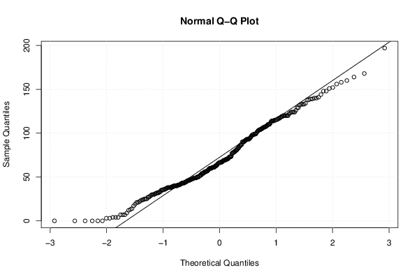
| Title produced by software | Linear Regression Graphical Model Validation | ||||||||||||||||||||||||||||||||||||||||||||||||||||||||||||
| Date of computation | Sun, 02 Dec 2012 09:14:16 -0500 | ||||||||||||||||||||||||||||||||||||||||||||||||||||||||||||
| Cite this page as follows | Statistical Computations at FreeStatistics.org, Office for Research Development and Education, URL https://freestatistics.org/blog/index.php?v=date/2012/Dec/02/t135445770083aa06legysqw1j.htm/, Retrieved Thu, 25 Apr 2024 23:18:28 +0000 | ||||||||||||||||||||||||||||||||||||||||||||||||||||||||||||
| Statistical Computations at FreeStatistics.org, Office for Research Development and Education, URL https://freestatistics.org/blog/index.php?pk=195517, Retrieved Thu, 25 Apr 2024 23:18:28 +0000 | |||||||||||||||||||||||||||||||||||||||||||||||||||||||||||||
| QR Codes: | |||||||||||||||||||||||||||||||||||||||||||||||||||||||||||||
|
| |||||||||||||||||||||||||||||||||||||||||||||||||||||||||||||
| Original text written by user: | |||||||||||||||||||||||||||||||||||||||||||||||||||||||||||||
| IsPrivate? | No (this computation is public) | ||||||||||||||||||||||||||||||||||||||||||||||||||||||||||||
| User-defined keywords | |||||||||||||||||||||||||||||||||||||||||||||||||||||||||||||
| Estimated Impact | 141 | ||||||||||||||||||||||||||||||||||||||||||||||||||||||||||||
Tree of Dependent Computations | |||||||||||||||||||||||||||||||||||||||||||||||||||||||||||||
| Family? (F = Feedback message, R = changed R code, M = changed R Module, P = changed Parameters, D = changed Data) | |||||||||||||||||||||||||||||||||||||||||||||||||||||||||||||
| - [Linear Regression Graphical Model Validation] [Colombia Coffee -...] [2008-02-26 10:22:06] [74be16979710d4c4e7c6647856088456] - RM D [Linear Regression Graphical Model Validation] [simple regression...] [2012-12-02 12:55:42] [74be16979710d4c4e7c6647856088456] - D [Linear Regression Graphical Model Validation] [lineair regressio...] [2012-12-02 13:14:50] [74be16979710d4c4e7c6647856088456] - D [Linear Regression Graphical Model Validation] [simple lineair re...] [2012-12-02 14:14:16] [d41d8cd98f00b204e9800998ecf8427e] [Current] | |||||||||||||||||||||||||||||||||||||||||||||||||||||||||||||
| Feedback Forum | |||||||||||||||||||||||||||||||||||||||||||||||||||||||||||||
Post a new message | |||||||||||||||||||||||||||||||||||||||||||||||||||||||||||||
Dataset | |||||||||||||||||||||||||||||||||||||||||||||||||||||||||||||
| Dataseries X: | |||||||||||||||||||||||||||||||||||||||||||||||||||||||||||||
94 103 93 103 51 70 91 22 38 93 60 123 148 90 124 70 168 115 71 66 134 117 108 84 156 120 114 94 120 81 110 133 122 158 109 124 39 92 126 0 70 37 38 120 93 95 77 90 80 31 110 66 138 133 113 100 7 140 61 41 96 164 78 49 102 124 99 129 62 73 114 99 70 104 116 91 74 138 67 151 72 120 115 105 104 108 98 69 111 99 71 27 69 107 73 107 93 129 69 118 73 119 104 107 99 90 197 36 85 139 106 50 64 31 63 92 106 63 69 41 56 25 65 93 114 38 44 87 110 0 27 83 30 80 98 82 0 60 28 9 33 59 49 115 140 49 120 66 21 124 152 139 38 144 120 160 114 39 78 119 141 101 56 133 83 116 90 36 50 61 97 98 78 117 148 41 105 55 132 44 21 50 0 73 86 0 13 4 57 48 46 48 32 68 87 43 67 46 46 56 48 44 60 65 55 38 52 60 54 86 24 52 49 61 61 81 43 40 40 56 68 79 47 57 41 29 3 60 30 79 47 40 48 36 42 49 57 12 40 43 33 77 43 45 47 43 45 50 35 7 71 67 0 62 54 4 25 40 38 19 17 67 14 30 54 35 59 24 58 42 46 61 3 52 25 40 32 4 49 63 67 32 23 7 54 37 35 51 39 | |||||||||||||||||||||||||||||||||||||||||||||||||||||||||||||
| Dataseries Y: | |||||||||||||||||||||||||||||||||||||||||||||||||||||||||||||
30 28 38 30 22 26 25 18 11 26 25 38 44 30 40 34 47 30 31 23 36 36 30 25 39 34 31 31 33 25 33 35 42 43 30 33 13 32 36 0 28 14 17 32 30 35 20 28 28 39 34 26 39 39 33 28 4 39 18 14 29 44 21 16 28 35 28 38 23 36 32 29 25 27 36 28 23 40 23 40 28 34 33 28 34 30 33 22 38 26 35 8 24 29 20 29 45 37 33 33 25 32 29 28 28 31 52 21 24 41 33 32 19 20 31 31 32 18 23 17 20 12 17 30 31 10 13 22 42 1 9 32 11 25 36 31 0 24 13 8 13 19 18 33 40 22 38 24 8 35 43 43 14 41 38 45 31 13 28 31 40 30 16 37 30 35 32 27 20 18 31 31 21 39 41 13 32 18 39 14 7 17 0 30 37 0 5 1 16 32 24 17 11 24 22 12 19 13 17 15 16 24 15 17 18 20 16 16 18 22 8 17 18 16 23 22 13 13 16 16 20 22 17 18 17 12 7 17 14 23 17 14 15 17 21 18 18 17 17 16 15 21 16 14 15 17 15 15 10 6 22 21 1 18 17 4 10 16 16 9 16 17 7 15 14 14 18 12 16 21 19 16 1 16 10 19 12 2 14 17 19 14 11 4 16 20 12 15 16 | |||||||||||||||||||||||||||||||||||||||||||||||||||||||||||||
Tables (Output of Computation) | |||||||||||||||||||||||||||||||||||||||||||||||||||||||||||||
| |||||||||||||||||||||||||||||||||||||||||||||||||||||||||||||
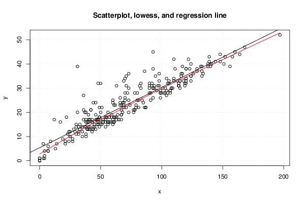
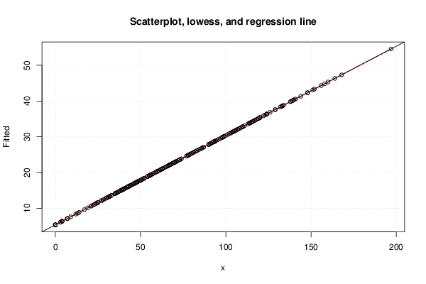
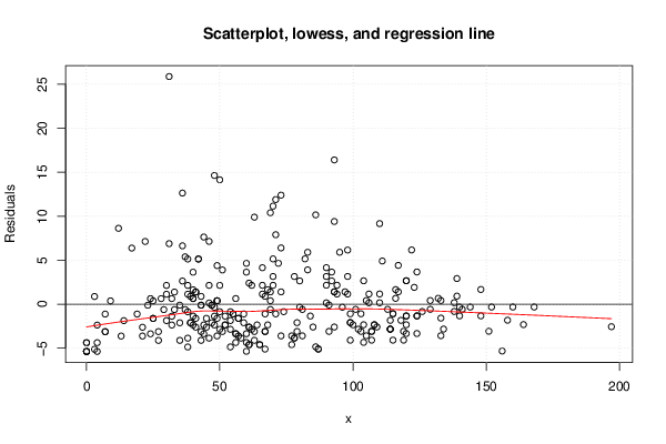
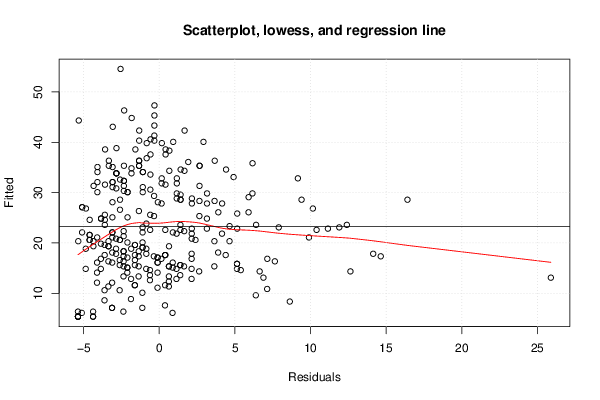
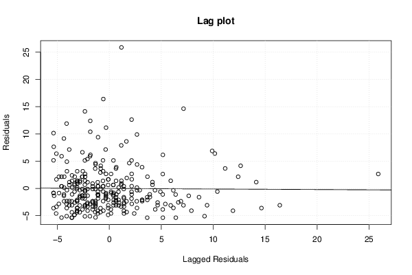
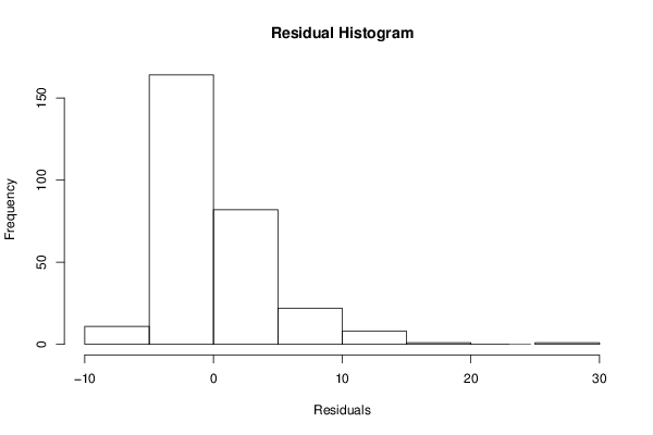
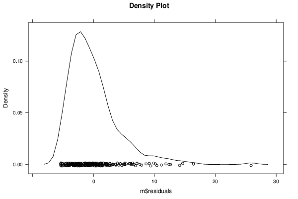
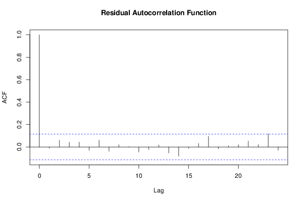
Figures (Output of Computation) | |||||||||||||||||||||||||||||||||||||||||||||||||||||||||||||
Input Parameters & R Code | |||||||||||||||||||||||||||||||||||||||||||||||||||||||||||||
| Parameters (Session): | |||||||||||||||||||||||||||||||||||||||||||||||||||||||||||||
| par1 = 0 ; | |||||||||||||||||||||||||||||||||||||||||||||||||||||||||||||
| Parameters (R input): | |||||||||||||||||||||||||||||||||||||||||||||||||||||||||||||
| par1 = 0 ; | |||||||||||||||||||||||||||||||||||||||||||||||||||||||||||||
| R code (references can be found in the software module): | |||||||||||||||||||||||||||||||||||||||||||||||||||||||||||||
par1 <- as.numeric(par1) | |||||||||||||||||||||||||||||||||||||||||||||||||||||||||||||