Repository of Reproducible Computations

Free Statistics

of Irreproducible Research!

Author's title

Author

*The author of this computation has been verified*

R Software Module

rwasp_autocorrelation.wasp

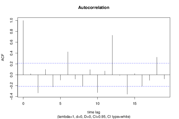
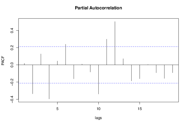
Title produced by software

(Partial) Autocorrelation Function

Date of computation

Sun, 02 Dec 2012 05:24:05 -0500

Cite this page as follows

Statistical Computations at FreeStatistics.org, Office for Research Development and Education, URL https://freestatistics.org/blog/index.php?v=date/2012/Dec/02/t1354443865zkjh2bp2ilit8fv.htm/, Retrieved Tue, 23 Apr 2024 22:29:05 +0000

Statistical Computations at FreeStatistics.org, Office for Research Development and Education, URL https://freestatistics.org/blog/index.php?pk=195407, Retrieved Tue, 23 Apr 2024 22:29:05 +0000

QR Codes:

Paste this QR Code to cite your computation.

Original text written by user:

IsPrivate?

No (this computation is public)

User-defined keywords

Estimated Impact

127

Family? (F = Feedback message, R = changed R code, M = changed R Module, P = changed Parameters, D = changed Data)

-     [Univariate Data Series] [data set] [2008-12-01 19:54:57] [b98453cac15ba1066b407e146608df68]
- RMP   [(Partial) Autocorrelation Function] [Unemployment] [2010-11-29 09:05:21] [b98453cac15ba1066b407e146608df68]
- R  D      [(Partial) Autocorrelation Function] [ws9] [2012-12-02 10:24:05] [2bcb0f1dab9cffb75c9fd882cacbd29a] [Current]
-   PD        [(Partial) Autocorrelation Function] [ws9] [2012-12-02 10:34:31] [7722d8427d2b2c713c1f0d5525f2f86c] 

Feedback Forum

Post a new message

Dataseries X:

Download CSV

Histogram

Boxplots

Summary of computational transaction
Raw Input	view raw input (R code)
Raw Output	view raw output of R engine
Computing time	2 seconds
R Server	'Gertrude Mary Cox' @ cox.wessa.net

\begin{tabular}{lllllllll}
\hline
Summary of computational transaction \tabularnewline
Raw Input & view raw input (R code)  \tabularnewline
Raw Output & view raw output of R engine  \tabularnewline
Computing time & 2 seconds \tabularnewline
R Server & 'Gertrude Mary Cox' @ cox.wessa.net \tabularnewline
\hline
\end{tabular}
%Source: https://freestatistics.org/blog/index.php?pk=195407&T=0

[TABLE]
[ROW][C]Summary of computational transaction[/C][/ROW]
[ROW][C]Raw Input[/C][C]view raw input (R code) [/C][/ROW]
[ROW][C]Raw Output[/C][C]view raw output of R engine [/C][/ROW]
[ROW][C]Computing time[/C][C]2 seconds[/C][/ROW]
[ROW][C]R Server[/C][C]'Gertrude Mary Cox' @ cox.wessa.net[/C][/ROW]
[/TABLE]
Source: https://freestatistics.org/blog/index.php?pk=195407&T=0

Globally Unique Identifier (entire table): ba.freestatistics.org/blog/index.php?pk=195407&T=0

As an alternative you can also use a QR Code:

The GUIDs for individual cells are displayed in the table below:

Summary of computational transaction
Raw Input	view raw input (R code)
Raw Output	view raw output of R engine
Computing time	2 seconds
R Server	'Gertrude Mary Cox' @ cox.wessa.net

Autocorrelation Function
Time lag k	ACF(k)	T-STAT	P-value
1	0.01783	0.1644	0.434908
2	-0.335341	-3.0917	0.001346
3	0.099014	0.9129	0.181948
4	-0.222914	-2.0552	0.021466
5	-0.098587	-0.9089	0.182978
6	0.422431	3.8946	9.8e-05
7	-0.07947	-0.7327	0.232887
8	-0.21229	-1.9572	0.026802
9	0.094574	0.8719	0.192852
10	-0.329475	-3.0376	0.001583
11	0.068597	0.6324	0.264402
12	0.728048	6.7123	0
13	-0.012206	-0.1125	0.455333
14	-0.358215	-3.3026	0.000701
15	0.021884	0.2018	0.420292
16	-0.210564	-1.9413	0.027767
17	-0.103158	-0.9511	0.172134
18	0.324135	2.9884	0.001833
19	-0.077199	-0.7117	0.239287

\begin{tabular}{lllllllll}
\hline
Autocorrelation Function \tabularnewline
Time lag k & ACF(k) & T-STAT & P-value \tabularnewline
1 & 0.01783 & 0.1644 & 0.434908 \tabularnewline
2 & -0.335341 & -3.0917 & 0.001346 \tabularnewline
3 & 0.099014 & 0.9129 & 0.181948 \tabularnewline
4 & -0.222914 & -2.0552 & 0.021466 \tabularnewline
5 & -0.098587 & -0.9089 & 0.182978 \tabularnewline
6 & 0.422431 & 3.8946 & 9.8e-05 \tabularnewline
7 & -0.07947 & -0.7327 & 0.232887 \tabularnewline
8 & -0.21229 & -1.9572 & 0.026802 \tabularnewline
9 & 0.094574 & 0.8719 & 0.192852 \tabularnewline
10 & -0.329475 & -3.0376 & 0.001583 \tabularnewline
11 & 0.068597 & 0.6324 & 0.264402 \tabularnewline
12 & 0.728048 & 6.7123 & 0 \tabularnewline
13 & -0.012206 & -0.1125 & 0.455333 \tabularnewline
14 & -0.358215 & -3.3026 & 0.000701 \tabularnewline
15 & 0.021884 & 0.2018 & 0.420292 \tabularnewline
16 & -0.210564 & -1.9413 & 0.027767 \tabularnewline
17 & -0.103158 & -0.9511 & 0.172134 \tabularnewline
18 & 0.324135 & 2.9884 & 0.001833 \tabularnewline
19 & -0.077199 & -0.7117 & 0.239287 \tabularnewline
\hline
\end{tabular}
%Source: https://freestatistics.org/blog/index.php?pk=195407&T=1

[TABLE]
[ROW][C]Autocorrelation Function[/C][/ROW]
[ROW][C]Time lag k[/C][C]ACF(k)[/C][C]T-STAT[/C][C]P-value[/C][/ROW]
[ROW][C]1[/C][C]0.01783[/C][C]0.1644[/C][C]0.434908[/C][/ROW]
[ROW][C]2[/C][C]-0.335341[/C][C]-3.0917[/C][C]0.001346[/C][/ROW]
[ROW][C]3[/C][C]0.099014[/C][C]0.9129[/C][C]0.181948[/C][/ROW]
[ROW][C]4[/C][C]-0.222914[/C][C]-2.0552[/C][C]0.021466[/C][/ROW]
[ROW][C]5[/C][C]-0.098587[/C][C]-0.9089[/C][C]0.182978[/C][/ROW]
[ROW][C]6[/C][C]0.422431[/C][C]3.8946[/C][C]9.8e-05[/C][/ROW]
[ROW][C]7[/C][C]-0.07947[/C][C]-0.7327[/C][C]0.232887[/C][/ROW]
[ROW][C]8[/C][C]-0.21229[/C][C]-1.9572[/C][C]0.026802[/C][/ROW]
[ROW][C]9[/C][C]0.094574[/C][C]0.8719[/C][C]0.192852[/C][/ROW]
[ROW][C]10[/C][C]-0.329475[/C][C]-3.0376[/C][C]0.001583[/C][/ROW]
[ROW][C]11[/C][C]0.068597[/C][C]0.6324[/C][C]0.264402[/C][/ROW]
[ROW][C]12[/C][C]0.728048[/C][C]6.7123[/C][C]0[/C][/ROW]
[ROW][C]13[/C][C]-0.012206[/C][C]-0.1125[/C][C]0.455333[/C][/ROW]
[ROW][C]14[/C][C]-0.358215[/C][C]-3.3026[/C][C]0.000701[/C][/ROW]
[ROW][C]15[/C][C]0.021884[/C][C]0.2018[/C][C]0.420292[/C][/ROW]
[ROW][C]16[/C][C]-0.210564[/C][C]-1.9413[/C][C]0.027767[/C][/ROW]
[ROW][C]17[/C][C]-0.103158[/C][C]-0.9511[/C][C]0.172134[/C][/ROW]
[ROW][C]18[/C][C]0.324135[/C][C]2.9884[/C][C]0.001833[/C][/ROW]
[ROW][C]19[/C][C]-0.077199[/C][C]-0.7117[/C][C]0.239287[/C][/ROW]
[/TABLE]
Source: https://freestatistics.org/blog/index.php?pk=195407&T=1

Globally Unique Identifier (entire table): ba.freestatistics.org/blog/index.php?pk=195407&T=1

As an alternative you can also use a QR Code:

The GUIDs for individual cells are displayed in the table below:

Autocorrelation Function
Time lag k	ACF(k)	T-STAT	P-value
1	0.01783	0.1644	0.434908
2	-0.335341	-3.0917	0.001346
3	0.099014	0.9129	0.181948
4	-0.222914	-2.0552	0.021466
5	-0.098587	-0.9089	0.182978
6	0.422431	3.8946	9.8e-05
7	-0.07947	-0.7327	0.232887
8	-0.21229	-1.9572	0.026802
9	0.094574	0.8719	0.192852
10	-0.329475	-3.0376	0.001583
11	0.068597	0.6324	0.264402
12	0.728048	6.7123	0
13	-0.012206	-0.1125	0.455333
14	-0.358215	-3.3026	0.000701
15	0.021884	0.2018	0.420292
16	-0.210564	-1.9413	0.027767
17	-0.103158	-0.9511	0.172134
18	0.324135	2.9884	0.001833
19	-0.077199	-0.7117	0.239287

Partial Autocorrelation Function
Time lag k	PACF(k)	T-STAT	P-value
1	0.01783	0.1644	0.434908
2	-0.335766	-3.0956	0.00133
3	0.127385	1.1744	0.121751
4	-0.395825	-3.6493	0.000226
5	0.044755	0.4126	0.340462
6	0.239861	2.2114	0.014846
7	-0.16155	-1.4894	0.07004
8	0.009437	0.087	0.465436
9	-0.082962	-0.7649	0.223232
10	-0.338538	-3.1212	0.001231
11	0.29898	2.7565	0.003575
12	0.503369	4.6408	6e-06
13	0.071682	0.6609	0.255239
14	-0.186118	-1.7159	0.04491
15	-0.16146	-1.4886	0.070149
16	0.004167	0.0384	0.484721
17	-0.091622	-0.8447	0.200321
18	-0.157749	-1.4544	0.074762
19	-0.091236	-0.8412	0.20131

\begin{tabular}{lllllllll}
\hline
Partial Autocorrelation Function \tabularnewline
Time lag k & PACF(k) & T-STAT & P-value \tabularnewline
1 & 0.01783 & 0.1644 & 0.434908 \tabularnewline
2 & -0.335766 & -3.0956 & 0.00133 \tabularnewline
3 & 0.127385 & 1.1744 & 0.121751 \tabularnewline
4 & -0.395825 & -3.6493 & 0.000226 \tabularnewline
5 & 0.044755 & 0.4126 & 0.340462 \tabularnewline
6 & 0.239861 & 2.2114 & 0.014846 \tabularnewline
7 & -0.16155 & -1.4894 & 0.07004 \tabularnewline
8 & 0.009437 & 0.087 & 0.465436 \tabularnewline
9 & -0.082962 & -0.7649 & 0.223232 \tabularnewline
10 & -0.338538 & -3.1212 & 0.001231 \tabularnewline
11 & 0.29898 & 2.7565 & 0.003575 \tabularnewline
12 & 0.503369 & 4.6408 & 6e-06 \tabularnewline
13 & 0.071682 & 0.6609 & 0.255239 \tabularnewline
14 & -0.186118 & -1.7159 & 0.04491 \tabularnewline
15 & -0.16146 & -1.4886 & 0.070149 \tabularnewline
16 & 0.004167 & 0.0384 & 0.484721 \tabularnewline
17 & -0.091622 & -0.8447 & 0.200321 \tabularnewline
18 & -0.157749 & -1.4544 & 0.074762 \tabularnewline
19 & -0.091236 & -0.8412 & 0.20131 \tabularnewline
\hline
\end{tabular}
%Source: https://freestatistics.org/blog/index.php?pk=195407&T=2

[TABLE]
[ROW][C]Partial Autocorrelation Function[/C][/ROW]
[ROW][C]Time lag k[/C][C]PACF(k)[/C][C]T-STAT[/C][C]P-value[/C][/ROW]
[ROW][C]1[/C][C]0.01783[/C][C]0.1644[/C][C]0.434908[/C][/ROW]
[ROW][C]2[/C][C]-0.335766[/C][C]-3.0956[/C][C]0.00133[/C][/ROW]
[ROW][C]3[/C][C]0.127385[/C][C]1.1744[/C][C]0.121751[/C][/ROW]
[ROW][C]4[/C][C]-0.395825[/C][C]-3.6493[/C][C]0.000226[/C][/ROW]
[ROW][C]5[/C][C]0.044755[/C][C]0.4126[/C][C]0.340462[/C][/ROW]
[ROW][C]6[/C][C]0.239861[/C][C]2.2114[/C][C]0.014846[/C][/ROW]
[ROW][C]7[/C][C]-0.16155[/C][C]-1.4894[/C][C]0.07004[/C][/ROW]
[ROW][C]8[/C][C]0.009437[/C][C]0.087[/C][C]0.465436[/C][/ROW]
[ROW][C]9[/C][C]-0.082962[/C][C]-0.7649[/C][C]0.223232[/C][/ROW]
[ROW][C]10[/C][C]-0.338538[/C][C]-3.1212[/C][C]0.001231[/C][/ROW]
[ROW][C]11[/C][C]0.29898[/C][C]2.7565[/C][C]0.003575[/C][/ROW]
[ROW][C]12[/C][C]0.503369[/C][C]4.6408[/C][C]6e-06[/C][/ROW]
[ROW][C]13[/C][C]0.071682[/C][C]0.6609[/C][C]0.255239[/C][/ROW]
[ROW][C]14[/C][C]-0.186118[/C][C]-1.7159[/C][C]0.04491[/C][/ROW]
[ROW][C]15[/C][C]-0.16146[/C][C]-1.4886[/C][C]0.070149[/C][/ROW]
[ROW][C]16[/C][C]0.004167[/C][C]0.0384[/C][C]0.484721[/C][/ROW]
[ROW][C]17[/C][C]-0.091622[/C][C]-0.8447[/C][C]0.200321[/C][/ROW]
[ROW][C]18[/C][C]-0.157749[/C][C]-1.4544[/C][C]0.074762[/C][/ROW]
[ROW][C]19[/C][C]-0.091236[/C][C]-0.8412[/C][C]0.20131[/C][/ROW]
[/TABLE]
Source: https://freestatistics.org/blog/index.php?pk=195407&T=2

Globally Unique Identifier (entire table): ba.freestatistics.org/blog/index.php?pk=195407&T=2

As an alternative you can also use a QR Code:

The GUIDs for individual cells are displayed in the table below:

Partial Autocorrelation Function
Time lag k	PACF(k)	T-STAT	P-value
1	0.01783	0.1644	0.434908
2	-0.335766	-3.0956	0.00133
3	0.127385	1.1744	0.121751
4	-0.395825	-3.6493	0.000226
5	0.044755	0.4126	0.340462
6	0.239861	2.2114	0.014846
7	-0.16155	-1.4894	0.07004
8	0.009437	0.087	0.465436
9	-0.082962	-0.7649	0.223232
10	-0.338538	-3.1212	0.001231
11	0.29898	2.7565	0.003575
12	0.503369	4.6408	6e-06
13	0.071682	0.6609	0.255239
14	-0.186118	-1.7159	0.04491
15	-0.16146	-1.4886	0.070149
16	0.004167	0.0384	0.484721
17	-0.091622	-0.8447	0.200321
18	-0.157749	-1.4544	0.074762
19	-0.091236	-0.8412	0.20131

Figure 1

PNG link

Postscript link

PDF link

Figure 2

PNG link

Postscript link

PDF link

Parameters (Session):

par1 = Default ; par2 = 1 ; par3 = 0 ; par4 = 0 ; par5 = 12 ; par6 = White Noise ; par7 = 0.95 ;

Parameters (R input):

par1 = Default ; par2 = 1 ; par3 = 0 ; par4 = 0 ; par5 = 12 ; par6 = White Noise ; par7 = 0.95 ; par8 = ;

R code (references can be found in the software module):

if (par1 == 'Default') {
par1 = 10*log10(length(x))
} else {
par1 <- as.numeric(par1)
}
par2 <- as.numeric(par2)
par3 <- as.numeric(par3)
par4 <- as.numeric(par4)
par5 <- as.numeric(par5)
if (par6 == 'White Noise') par6 <- 'white' else par6 <- 'ma'
par7 <- as.numeric(par7)
if (par2 == 0) {
x <- log(x)
} else {
x <- (x ^ par2 - 1) / par2
}
if (par3 > 0) x <- diff(x,lag=1,difference=par3)
if (par4 > 0) x <- diff(x,lag=par5,difference=par4)
bitmap(file='pic1.png')
racf <- acf(x, par1, main='Autocorrelation', xlab='time lag', ylab='ACF', ci.type=par6, ci=par7, sub=paste('(lambda=',par2,', d=',par3,', D=',par4,', CI=', par7, ', CI type=',par6,')',sep=''))
dev.off()
bitmap(file='pic2.png')
rpacf <- pacf(x,par1,main='Partial Autocorrelation',xlab='lags',ylab='PACF')
dev.off()
(myacf <- c(racf$acf))
(mypacf <- c(rpacf$acf))
lengthx <- length(x)
sqrtn <- sqrt(lengthx)
load(file='createtable')
a<-table.start()
a<-table.row.start(a)
a<-table.element(a,'Autocorrelation Function',4,TRUE)
a<-table.row.end(a)
a<-table.row.start(a)
a<-table.element(a,'Time lag k',header=TRUE)
a<-table.element(a,hyperlink('basics.htm','ACF(k)','click here for more information about the Autocorrelation Function'),header=TRUE)
a<-table.element(a,'T-STAT',header=TRUE)
a<-table.element(a,'P-value',header=TRUE)
a<-table.row.end(a)
for (i in 2:(par1+1)) {
a<-table.row.start(a)
a<-table.element(a,i-1,header=TRUE)
a<-table.element(a,round(myacf[i],6))
mytstat <- myacf[i]*sqrtn
a<-table.element(a,round(mytstat,4))
a<-table.element(a,round(1-pt(abs(mytstat),lengthx),6))
a<-table.row.end(a)
}
a<-table.end(a)
table.save(a,file='mytable.tab')
a<-table.start()
a<-table.row.start(a)
a<-table.element(a,'Partial Autocorrelation Function',4,TRUE)
a<-table.row.end(a)
a<-table.row.start(a)
a<-table.element(a,'Time lag k',header=TRUE)
a<-table.element(a,hyperlink('basics.htm','PACF(k)','click here for more information about the Partial Autocorrelation Function'),header=TRUE)
a<-table.element(a,'T-STAT',header=TRUE)
a<-table.element(a,'P-value',header=TRUE)
a<-table.row.end(a)
for (i in 1:par1) {
a<-table.row.start(a)
a<-table.element(a,i,header=TRUE)
a<-table.element(a,round(mypacf[i],6))
mytstat <- mypacf[i]*sqrtn
a<-table.element(a,round(mytstat,4))
a<-table.element(a,round(1-pt(abs(mytstat),lengthx),6))
a<-table.row.end(a)
}
a<-table.end(a)
table.save(a,file='mytable1.tab')

Free Statistics

Description of Statistical Computation

Tree of Dependent Computations

Dataset

Tables (Output of Computation)

Figures (Output of Computation)

Input Parameters & R Code