Repository of Reproducible Computations

Free Statistics

of Irreproducible Research!

Author's title

Author

*The author of this computation has been verified*

R Software Module

rwasp_autocorrelation.wasp

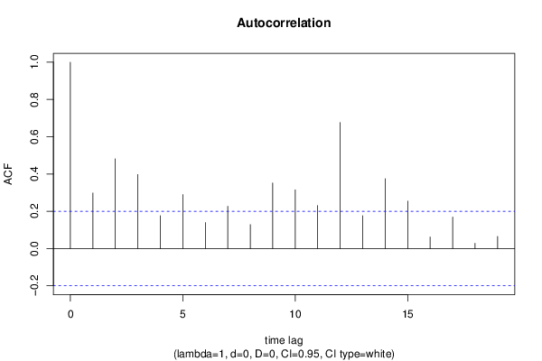
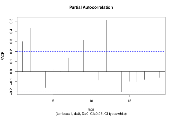
Title produced by software

(Partial) Autocorrelation Function

Date of computation

Sat, 01 Dec 2012 07:28:25 -0500

Cite this page as follows

Statistical Computations at FreeStatistics.org, Office for Research Development and Education, URL https://freestatistics.org/blog/index.php?v=date/2012/Dec/01/t13543649923kz89jag8l6hj0j.htm/, Retrieved Mon, 29 Apr 2024 06:40:51 +0000

Statistical Computations at FreeStatistics.org, Office for Research Development and Education, URL https://freestatistics.org/blog/index.php?pk=195262, Retrieved Mon, 29 Apr 2024 06:40:51 +0000

QR Codes:

Paste this QR Code to cite your computation.

Original text written by user:

IsPrivate?

No (this computation is public)

User-defined keywords

Estimated Impact

191

Family? (F = Feedback message, R = changed R code, M = changed R Module, P = changed Parameters, D = changed Data)

-     [Univariate Data Series] [Paper - exogene v...] [2010-12-01 16:02:49] [6f0e7a2d1a07390e3505a2db8288f975]
- RMP     [(Partial) Autocorrelation Function] [ACF 1] [2012-12-01 12:28:25] [4289cf790da1cc09a0cb8798de13fde3] [Current]
- R P       [(Partial) Autocorrelation Function] [ACF 2] [2012-12-01 12:32:22] [aa4758794357e809405bf1fb1497cdc4] 
-   P       [(Partial) Autocorrelation Function] [ACF 3] [2012-12-01 12:34:12] [aa4758794357e809405bf1fb1497cdc4] 
- RMP       [Spectral Analysis] [Spectral Analysis] [2012-12-01 12:37:54] [aa4758794357e809405bf1fb1497cdc4] 
- R           [Spectral Analysis] [spectral analysis 2] [2012-12-20 16:02:31] [77d02b0cf2cecd023ffa9a06f056f18d] 
- RMP       [Spectral Analysis] [Spectral Analysis 2] [2012-12-01 12:42:46] [aa4758794357e809405bf1fb1497cdc4] 
- RMP       [Variance Reduction Matrix] [VRM] [2012-12-01 12:45:23] [aa4758794357e809405bf1fb1497cdc4] 
- RMP       [Standard Deviation-Mean Plot] [SMP] [2012-12-01 12:57:14] [aa4758794357e809405bf1fb1497cdc4] 
- RMP       [ARIMA Backward Selection] [ARIMA] [2012-12-01 13:04:22] [aa4758794357e809405bf1fb1497cdc4] 
- RMP       [ARIMA Forecasting] [ARIMA Forecast] [2012-12-01 13:15:00] [aa4758794357e809405bf1fb1497cdc4] 
- R P         [ARIMA Forecasting] [Geboortes Forecast] [2012-12-14 19:36:28] [aa4758794357e809405bf1fb1497cdc4] 

Feedback Forum

Post a new message

Dataseries X:

Download CSV

Histogram

Boxplots

Summary of computational transaction
Raw Input	view raw input (R code)
Raw Output	view raw output of R engine
Computing time	3 seconds
R Server	'Gertrude Mary Cox' @ cox.wessa.net

\begin{tabular}{lllllllll}
\hline
Summary of computational transaction \tabularnewline
Raw Input & view raw input (R code)  \tabularnewline
Raw Output & view raw output of R engine  \tabularnewline
Computing time & 3 seconds \tabularnewline
R Server & 'Gertrude Mary Cox' @ cox.wessa.net \tabularnewline
\hline
\end{tabular}
%Source: https://freestatistics.org/blog/index.php?pk=195262&T=0

[TABLE]
[ROW][C]Summary of computational transaction[/C][/ROW]
[ROW][C]Raw Input[/C][C]view raw input (R code) [/C][/ROW]
[ROW][C]Raw Output[/C][C]view raw output of R engine [/C][/ROW]
[ROW][C]Computing time[/C][C]3 seconds[/C][/ROW]
[ROW][C]R Server[/C][C]'Gertrude Mary Cox' @ cox.wessa.net[/C][/ROW]
[/TABLE]
Source: https://freestatistics.org/blog/index.php?pk=195262&T=0

Globally Unique Identifier (entire table): ba.freestatistics.org/blog/index.php?pk=195262&T=0

As an alternative you can also use a QR Code:

The GUIDs for individual cells are displayed in the table below:

Summary of computational transaction
Raw Input	view raw input (R code)
Raw Output	view raw output of R engine
Computing time	3 seconds
R Server	'Gertrude Mary Cox' @ cox.wessa.net

Autocorrelation Function
Time lag k	ACF(k)	T-STAT	P-value
1	0.297897	2.9188	0.002189
2	0.481692	4.7196	4e-06
3	0.397353	3.8932	9.1e-05
4	0.176272	1.7271	0.043682
5	0.289332	2.8349	0.002795
6	0.139249	1.3644	0.087823
7	0.226553	2.2198	0.014395
8	0.128357	1.2576	0.105787
9	0.352086	3.4497	0.000418
10	0.314914	3.0855	0.001327
11	0.230382	2.2573	0.013129
12	0.676174	6.6251	0
13	0.176392	1.7283	0.043576
14	0.374695	3.6712	0.000198
15	0.254251	2.4911	0.007225
16	0.061614	0.6037	0.273738
17	0.169198	1.6578	0.050311
18	0.02778	0.2722	0.39303
19	0.065024	0.6371	0.262786

\begin{tabular}{lllllllll}
\hline
Autocorrelation Function \tabularnewline
Time lag k & ACF(k) & T-STAT & P-value \tabularnewline
1 & 0.297897 & 2.9188 & 0.002189 \tabularnewline
2 & 0.481692 & 4.7196 & 4e-06 \tabularnewline
3 & 0.397353 & 3.8932 & 9.1e-05 \tabularnewline
4 & 0.176272 & 1.7271 & 0.043682 \tabularnewline
5 & 0.289332 & 2.8349 & 0.002795 \tabularnewline
6 & 0.139249 & 1.3644 & 0.087823 \tabularnewline
7 & 0.226553 & 2.2198 & 0.014395 \tabularnewline
8 & 0.128357 & 1.2576 & 0.105787 \tabularnewline
9 & 0.352086 & 3.4497 & 0.000418 \tabularnewline
10 & 0.314914 & 3.0855 & 0.001327 \tabularnewline
11 & 0.230382 & 2.2573 & 0.013129 \tabularnewline
12 & 0.676174 & 6.6251 & 0 \tabularnewline
13 & 0.176392 & 1.7283 & 0.043576 \tabularnewline
14 & 0.374695 & 3.6712 & 0.000198 \tabularnewline
15 & 0.254251 & 2.4911 & 0.007225 \tabularnewline
16 & 0.061614 & 0.6037 & 0.273738 \tabularnewline
17 & 0.169198 & 1.6578 & 0.050311 \tabularnewline
18 & 0.02778 & 0.2722 & 0.39303 \tabularnewline
19 & 0.065024 & 0.6371 & 0.262786 \tabularnewline
\hline
\end{tabular}
%Source: https://freestatistics.org/blog/index.php?pk=195262&T=1

[TABLE]
[ROW][C]Autocorrelation Function[/C][/ROW]
[ROW][C]Time lag k[/C][C]ACF(k)[/C][C]T-STAT[/C][C]P-value[/C][/ROW]
[ROW][C]1[/C][C]0.297897[/C][C]2.9188[/C][C]0.002189[/C][/ROW]
[ROW][C]2[/C][C]0.481692[/C][C]4.7196[/C][C]4e-06[/C][/ROW]
[ROW][C]3[/C][C]0.397353[/C][C]3.8932[/C][C]9.1e-05[/C][/ROW]
[ROW][C]4[/C][C]0.176272[/C][C]1.7271[/C][C]0.043682[/C][/ROW]
[ROW][C]5[/C][C]0.289332[/C][C]2.8349[/C][C]0.002795[/C][/ROW]
[ROW][C]6[/C][C]0.139249[/C][C]1.3644[/C][C]0.087823[/C][/ROW]
[ROW][C]7[/C][C]0.226553[/C][C]2.2198[/C][C]0.014395[/C][/ROW]
[ROW][C]8[/C][C]0.128357[/C][C]1.2576[/C][C]0.105787[/C][/ROW]
[ROW][C]9[/C][C]0.352086[/C][C]3.4497[/C][C]0.000418[/C][/ROW]
[ROW][C]10[/C][C]0.314914[/C][C]3.0855[/C][C]0.001327[/C][/ROW]
[ROW][C]11[/C][C]0.230382[/C][C]2.2573[/C][C]0.013129[/C][/ROW]
[ROW][C]12[/C][C]0.676174[/C][C]6.6251[/C][C]0[/C][/ROW]
[ROW][C]13[/C][C]0.176392[/C][C]1.7283[/C][C]0.043576[/C][/ROW]
[ROW][C]14[/C][C]0.374695[/C][C]3.6712[/C][C]0.000198[/C][/ROW]
[ROW][C]15[/C][C]0.254251[/C][C]2.4911[/C][C]0.007225[/C][/ROW]
[ROW][C]16[/C][C]0.061614[/C][C]0.6037[/C][C]0.273738[/C][/ROW]
[ROW][C]17[/C][C]0.169198[/C][C]1.6578[/C][C]0.050311[/C][/ROW]
[ROW][C]18[/C][C]0.02778[/C][C]0.2722[/C][C]0.39303[/C][/ROW]
[ROW][C]19[/C][C]0.065024[/C][C]0.6371[/C][C]0.262786[/C][/ROW]
[/TABLE]
Source: https://freestatistics.org/blog/index.php?pk=195262&T=1

Globally Unique Identifier (entire table): ba.freestatistics.org/blog/index.php?pk=195262&T=1

As an alternative you can also use a QR Code:

The GUIDs for individual cells are displayed in the table below:

Autocorrelation Function
Time lag k	ACF(k)	T-STAT	P-value
1	0.297897	2.9188	0.002189
2	0.481692	4.7196	4e-06
3	0.397353	3.8932	9.1e-05
4	0.176272	1.7271	0.043682
5	0.289332	2.8349	0.002795
6	0.139249	1.3644	0.087823
7	0.226553	2.2198	0.014395
8	0.128357	1.2576	0.105787
9	0.352086	3.4497	0.000418
10	0.314914	3.0855	0.001327
11	0.230382	2.2573	0.013129
12	0.676174	6.6251	0
13	0.176392	1.7283	0.043576
14	0.374695	3.6712	0.000198
15	0.254251	2.4911	0.007225
16	0.061614	0.6037	0.273738
17	0.169198	1.6578	0.050311
18	0.02778	0.2722	0.39303
19	0.065024	0.6371	0.262786

Partial Autocorrelation Function
Time lag k	PACF(k)	T-STAT	P-value
1	0.297897	2.9188	0.002189
2	0.431217	4.225	2.7e-05
3	0.25246	2.4736	0.007566
4	-0.158542	-1.5534	0.06181
5	0.020347	0.1994	0.421202
6	0.002396	0.0235	0.490659
7	0.136959	1.3419	0.091394
8	-0.030663	-0.3004	0.382249
9	0.309389	3.0314	0.001565
10	0.217807	2.1341	0.017693
11	-0.086196	-0.8445	0.200233
12	0.51162	5.0128	1e-06
13	-0.171661	-1.6819	0.047917
14	-0.200985	-1.9692	0.025904
15	-0.097464	-0.9549	0.171002
16	-0.100373	-0.9835	0.163929
17	-0.078669	-0.7708	0.22136
18	-0.014127	-0.1384	0.4451
19	-0.059065	-0.5787	0.282069

\begin{tabular}{lllllllll}
\hline
Partial Autocorrelation Function \tabularnewline
Time lag k & PACF(k) & T-STAT & P-value \tabularnewline
1 & 0.297897 & 2.9188 & 0.002189 \tabularnewline
2 & 0.431217 & 4.225 & 2.7e-05 \tabularnewline
3 & 0.25246 & 2.4736 & 0.007566 \tabularnewline
4 & -0.158542 & -1.5534 & 0.06181 \tabularnewline
5 & 0.020347 & 0.1994 & 0.421202 \tabularnewline
6 & 0.002396 & 0.0235 & 0.490659 \tabularnewline
7 & 0.136959 & 1.3419 & 0.091394 \tabularnewline
8 & -0.030663 & -0.3004 & 0.382249 \tabularnewline
9 & 0.309389 & 3.0314 & 0.001565 \tabularnewline
10 & 0.217807 & 2.1341 & 0.017693 \tabularnewline
11 & -0.086196 & -0.8445 & 0.200233 \tabularnewline
12 & 0.51162 & 5.0128 & 1e-06 \tabularnewline
13 & -0.171661 & -1.6819 & 0.047917 \tabularnewline
14 & -0.200985 & -1.9692 & 0.025904 \tabularnewline
15 & -0.097464 & -0.9549 & 0.171002 \tabularnewline
16 & -0.100373 & -0.9835 & 0.163929 \tabularnewline
17 & -0.078669 & -0.7708 & 0.22136 \tabularnewline
18 & -0.014127 & -0.1384 & 0.4451 \tabularnewline
19 & -0.059065 & -0.5787 & 0.282069 \tabularnewline
\hline
\end{tabular}
%Source: https://freestatistics.org/blog/index.php?pk=195262&T=2

[TABLE]
[ROW][C]Partial Autocorrelation Function[/C][/ROW]
[ROW][C]Time lag k[/C][C]PACF(k)[/C][C]T-STAT[/C][C]P-value[/C][/ROW]
[ROW][C]1[/C][C]0.297897[/C][C]2.9188[/C][C]0.002189[/C][/ROW]
[ROW][C]2[/C][C]0.431217[/C][C]4.225[/C][C]2.7e-05[/C][/ROW]
[ROW][C]3[/C][C]0.25246[/C][C]2.4736[/C][C]0.007566[/C][/ROW]
[ROW][C]4[/C][C]-0.158542[/C][C]-1.5534[/C][C]0.06181[/C][/ROW]
[ROW][C]5[/C][C]0.020347[/C][C]0.1994[/C][C]0.421202[/C][/ROW]
[ROW][C]6[/C][C]0.002396[/C][C]0.0235[/C][C]0.490659[/C][/ROW]
[ROW][C]7[/C][C]0.136959[/C][C]1.3419[/C][C]0.091394[/C][/ROW]
[ROW][C]8[/C][C]-0.030663[/C][C]-0.3004[/C][C]0.382249[/C][/ROW]
[ROW][C]9[/C][C]0.309389[/C][C]3.0314[/C][C]0.001565[/C][/ROW]
[ROW][C]10[/C][C]0.217807[/C][C]2.1341[/C][C]0.017693[/C][/ROW]
[ROW][C]11[/C][C]-0.086196[/C][C]-0.8445[/C][C]0.200233[/C][/ROW]
[ROW][C]12[/C][C]0.51162[/C][C]5.0128[/C][C]1e-06[/C][/ROW]
[ROW][C]13[/C][C]-0.171661[/C][C]-1.6819[/C][C]0.047917[/C][/ROW]
[ROW][C]14[/C][C]-0.200985[/C][C]-1.9692[/C][C]0.025904[/C][/ROW]
[ROW][C]15[/C][C]-0.097464[/C][C]-0.9549[/C][C]0.171002[/C][/ROW]
[ROW][C]16[/C][C]-0.100373[/C][C]-0.9835[/C][C]0.163929[/C][/ROW]
[ROW][C]17[/C][C]-0.078669[/C][C]-0.7708[/C][C]0.22136[/C][/ROW]
[ROW][C]18[/C][C]-0.014127[/C][C]-0.1384[/C][C]0.4451[/C][/ROW]
[ROW][C]19[/C][C]-0.059065[/C][C]-0.5787[/C][C]0.282069[/C][/ROW]
[/TABLE]
Source: https://freestatistics.org/blog/index.php?pk=195262&T=2

Globally Unique Identifier (entire table): ba.freestatistics.org/blog/index.php?pk=195262&T=2

As an alternative you can also use a QR Code:

The GUIDs for individual cells are displayed in the table below:

Partial Autocorrelation Function
Time lag k	PACF(k)	T-STAT	P-value
1	0.297897	2.9188	0.002189
2	0.431217	4.225	2.7e-05
3	0.25246	2.4736	0.007566
4	-0.158542	-1.5534	0.06181
5	0.020347	0.1994	0.421202
6	0.002396	0.0235	0.490659
7	0.136959	1.3419	0.091394
8	-0.030663	-0.3004	0.382249
9	0.309389	3.0314	0.001565
10	0.217807	2.1341	0.017693
11	-0.086196	-0.8445	0.200233
12	0.51162	5.0128	1e-06
13	-0.171661	-1.6819	0.047917
14	-0.200985	-1.9692	0.025904
15	-0.097464	-0.9549	0.171002
16	-0.100373	-0.9835	0.163929
17	-0.078669	-0.7708	0.22136
18	-0.014127	-0.1384	0.4451
19	-0.059065	-0.5787	0.282069

Figure 1

PNG link

Postscript link

PDF link

Figure 2

PNG link

Postscript link

PDF link

Figure 3

PNG link

Postscript link

PDF link

Parameters (Session):

par1 = Default ; par2 = 1 ; par3 = 0 ; par4 = 0 ; par5 = 12 ; par6 = White Noise ; par7 = 0.95 ;

Parameters (R input):

par1 = Default ; par2 = 1 ; par3 = 0 ; par4 = 0 ; par5 = 12 ; par6 = White Noise ; par7 = 0.95 ; par8 = ;

R code (references can be found in the software module):

if (par1 == 'Default') {
par1 = 10*log10(length(x))
} else {
par1 <- as.numeric(par1)
}
par2 <- as.numeric(par2)
par3 <- as.numeric(par3)
par4 <- as.numeric(par4)
par5 <- as.numeric(par5)
if (par6 == 'White Noise') par6 <- 'white' else par6 <- 'ma'
par7 <- as.numeric(par7)
if (par8 != '') par8 <- as.numeric(par8)
ox <- x
if (par8 == '') {
if (par2 == 0) {
x <- log(x)
} else {
x <- (x ^ par2 - 1) / par2
}
} else {
x <- log(x,base=par8)
}
if (par3 > 0) x <- diff(x,lag=1,difference=par3)
if (par4 > 0) x <- diff(x,lag=par5,difference=par4)
bitmap(file='picts.png')
op <- par(mfrow=c(2,1))
plot(ox,type='l',main='Original Time Series',xlab='time',ylab='value')
if (par8=='') {
mytitle <- paste('Working Time Series (lambda=',par2,', d=',par3,', D=',par4,')',sep='')
mysub <- paste('(lambda=',par2,', d=',par3,', D=',par4,', CI=', par7, ', CI type=',par6,')',sep='')
} else {
mytitle <- paste('Working Time Series (base=',par8,', d=',par3,', D=',par4,')',sep='')
mysub <- paste('(base=',par8,', d=',par3,', D=',par4,', CI=', par7, ', CI type=',par6,')',sep='')
}
plot(x,type='l', main=mytitle,xlab='time',ylab='value')
par(op)
dev.off()
bitmap(file='pic1.png')
racf <- acf(x, par1, main='Autocorrelation', xlab='time lag', ylab='ACF', ci.type=par6, ci=par7, sub=mysub)
dev.off()
bitmap(file='pic2.png')
rpacf <- pacf(x,par1,main='Partial Autocorrelation',xlab='lags',ylab='PACF',sub=mysub)
dev.off()
(myacf <- c(racf$acf))
(mypacf <- c(rpacf$acf))
lengthx <- length(x)
sqrtn <- sqrt(lengthx)
load(file='createtable')
a<-table.start()
a<-table.row.start(a)
a<-table.element(a,'Autocorrelation Function',4,TRUE)
a<-table.row.end(a)
a<-table.row.start(a)
a<-table.element(a,'Time lag k',header=TRUE)
a<-table.element(a,hyperlink('basics.htm','ACF(k)','click here for more information about the Autocorrelation Function'),header=TRUE)
a<-table.element(a,'T-STAT',header=TRUE)
a<-table.element(a,'P-value',header=TRUE)
a<-table.row.end(a)
for (i in 2:(par1+1)) {
a<-table.row.start(a)
a<-table.element(a,i-1,header=TRUE)
a<-table.element(a,round(myacf[i],6))
mytstat <- myacf[i]*sqrtn
a<-table.element(a,round(mytstat,4))
a<-table.element(a,round(1-pt(abs(mytstat),lengthx),6))
a<-table.row.end(a)
}
a<-table.end(a)
table.save(a,file='mytable.tab')
a<-table.start()
a<-table.row.start(a)
a<-table.element(a,'Partial Autocorrelation Function',4,TRUE)
a<-table.row.end(a)
a<-table.row.start(a)
a<-table.element(a,'Time lag k',header=TRUE)
a<-table.element(a,hyperlink('basics.htm','PACF(k)','click here for more information about the Partial Autocorrelation Function'),header=TRUE)
a<-table.element(a,'T-STAT',header=TRUE)
a<-table.element(a,'P-value',header=TRUE)
a<-table.row.end(a)
for (i in 1:par1) {
a<-table.row.start(a)
a<-table.element(a,i,header=TRUE)
a<-table.element(a,round(mypacf[i],6))
mytstat <- mypacf[i]*sqrtn
a<-table.element(a,round(mytstat,4))
a<-table.element(a,round(1-pt(abs(mytstat),lengthx),6))
a<-table.row.end(a)
}
a<-table.end(a)
table.save(a,file='mytable1.tab')

Free Statistics

Description of Statistical Computation

Tree of Dependent Computations

Dataset

Tables (Output of Computation)

Figures (Output of Computation)

Input Parameters & R Code