Free Statistics

of Irreproducible Research!

Author's title

Author*The author of this computation has been verified*
R Software Modulerwasp_bidensity.wasp
Title produced by softwareBivariate Kernel Density Estimation
Date of computationWed, 30 Nov 2011 09:52:33 -0500
Cite this page as followsStatistical Computations at FreeStatistics.org, Office for Research Development and Education, URL https://freestatistics.org/blog/index.php?v=date/2011/Nov/30/t1322664761o757r9aov7shieo.htm/, Retrieved Fri, 26 Apr 2024 02:32:34 +0000
Statistical Computations at FreeStatistics.org, Office for Research Development and Education, URL https://freestatistics.org/blog/index.php?pk=149017, Retrieved Fri, 26 Apr 2024 02:32:34 +0000
QR Codes:

Original text written by user:
IsPrivate?No (this computation is public)
User-defined keywords
Estimated Impact92
Family? (F = Feedback message, R = changed R code, M = changed R Module, P = changed Parameters, D = changed Data)
-     [Kernel Density Estimation] [] [2011-11-30 14:45:46] [f98f9dc58dd24d7896d4ecb781e1c75c]
- RMPD  [Pearson Correlation] [] [2011-11-30 14:49:33] [f98f9dc58dd24d7896d4ecb781e1c75c]
- RMP       [Bivariate Kernel Density Estimation] [] [2011-11-30 14:52:33] [4cf172296f32adf71d8383c359dbb80f] [Current]
Feedback Forum

Post a new message
Dataseries X:
113
119
133
130
122
136
149
149
137
120
105
119
116
127
142
136
126
150
171
171
159
134
115
141
146
151
179
164
173
179
200
200
185
163
147
167
172
181
194
182
184
219
231
243
210
192
173
195
197
197
237
236
230
244
265
273
238
212
181
202
205
189
236
228
235
265
303
294
260
230
204
230
243
234
268
270
271
316
365
348
313
275
238
279
285
278
318
314
319
375
414
406
356
307
272
307
316
302
357
349
356
423
466
468
405
348
306
337
341
319
363
349
364
436
492
506
405
360
311
338
361
343
407
397
421
473
549
560
464
408
363
406
418
392
420
462
473
536
623
607
509
462
391
433
Dataseries Y:
112
118
132
129
121
135
148
148
136
119
104
118
115
126
141
135
125
149
170
170
158
133
114
140
145
150
178
163
172
178
199
199
184
162
146
166
171
180
193
181
183
218
230
242
209
191
172
194
196
196
236
235
229
243
264
272
237
211
180
201
204
188
235
227
234
264
302
293
259
229
203
229
242
233
267
269
270
315
364
347
312
274
237
278
284
277
317
313
318
374
413
405
355
306
271
306
315
301
356
348
355
422
465
467
404
347
305
336
340
318
362
348
363
435
491
505
404
359
310
337
360
342
406
396
420
472
548
559
463
407
362
405
417
391
419
461
472
535
622
606
508
461
390
432


Summary of computational transaction
Raw Inputview raw input (R code)
Raw Outputview raw output of R engine
Computing time2 seconds
R Server'AstonUniversity' @ aston.wessa.net

\begin{tabular}{lllllllll}
\hline
Summary of computational transaction \tabularnewline
Raw Input & view raw input (R code)  \tabularnewline
Raw Output & view raw output of R engine  \tabularnewline
Computing time & 2 seconds \tabularnewline
R Server & 'AstonUniversity' @ aston.wessa.net \tabularnewline
\hline
\end{tabular}
%Source: https://freestatistics.org/blog/index.php?pk=149017&T=0

[TABLE]
[ROW][C]Summary of computational transaction[/C][/ROW]
[ROW][C]Raw Input[/C][C]view raw input (R code) [/C][/ROW]
[ROW][C]Raw Output[/C][C]view raw output of R engine [/C][/ROW]
[ROW][C]Computing time[/C][C]2 seconds[/C][/ROW]
[ROW][C]R Server[/C][C]'AstonUniversity' @ aston.wessa.net[/C][/ROW]
[/TABLE]
Source: https://freestatistics.org/blog/index.php?pk=149017&T=0

Globally Unique Identifier (entire table): ba.freestatistics.org/blog/index.php?pk=149017&T=0

As an alternative you can also use a QR Code:  

The GUIDs for individual cells are displayed in the table below:

Summary of computational transaction
Raw Inputview raw input (R code)
Raw Outputview raw output of R engine
Computing time2 seconds
R Server'AstonUniversity' @ aston.wessa.net


Bandwidth
x axis37.1396563787684
y axis37.1396563787684
Correlation
correlation used in KDE1
correlation(x,y)1

\begin{tabular}{lllllllll}
\hline
Bandwidth \tabularnewline
x axis & 37.1396563787684 \tabularnewline
y axis & 37.1396563787684 \tabularnewline
Correlation \tabularnewline
correlation used in KDE & 1 \tabularnewline
correlation(x,y) & 1 \tabularnewline
\hline
\end{tabular}
%Source: https://freestatistics.org/blog/index.php?pk=149017&T=1

[TABLE]
[ROW][C]Bandwidth[/C][/ROW]
[ROW][C]x axis[/C][C]37.1396563787684[/C][/ROW]
[ROW][C]y axis[/C][C]37.1396563787684[/C][/ROW]
[ROW][C]Correlation[/C][/ROW]
[ROW][C]correlation used in KDE[/C][C]1[/C][/ROW]
[ROW][C]correlation(x,y)[/C][C]1[/C][/ROW]
[/TABLE]
Source: https://freestatistics.org/blog/index.php?pk=149017&T=1

Globally Unique Identifier (entire table): ba.freestatistics.org/blog/index.php?pk=149017&T=1

As an alternative you can also use a QR Code:  

The GUIDs for individual cells are displayed in the table below:

Bandwidth
x axis37.1396563787684
y axis37.1396563787684
Correlation
correlation used in KDE1
correlation(x,y)1


Parameters (Session):
par1 = 50 ; par2 = 50 ; par3 = 0 ; par4 = 0 ; par5 = 0 ; par6 = Y ; par7 = Y ; par8 = terrain.colors ;
Parameters (R input):
par1 = 50 ; par2 = 50 ; par3 = 0 ; par4 = 0 ; par5 = 0 ; par6 = Y ; par7 = Y ; par8 = terrain.colors ;
R code (references can be found in the software module):
par1 <- as(par1,'numeric')
par2 <- as(par2,'numeric')
par3 <- as(par3,'numeric')
par4 <- as(par4,'numeric')
par5 <- as(par5,'numeric')
library('GenKern')
if (par3==0) par3 <- dpik(x)
if (par4==0) par4 <- dpik(y)
if (par5==0) par5 <- cor(x,y)
if (par1 > 500) par1 <- 500
if (par2 > 500) par2 <- 500
if (par8 == 'terrain.colors') mycol <- terrain.colors(100)
if (par8 == 'rainbow') mycol <- rainbow(100)
if (par8 == 'heat.colors') mycol <- heat.colors(100)
if (par8 == 'topo.colors') mycol <- topo.colors(100)
if (par8 == 'cm.colors') mycol <- cm.colors(100)
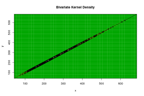
bitmap(file='bidensity.png')
op <- KernSur(x,y, xgridsize=par1, ygridsize=par2, correlation=par5, xbandwidth=par3, ybandwidth=par4)
image(op$xords, op$yords, op$zden, col=mycol, axes=TRUE,main=main,xlab=xlab,ylab=ylab)
if (par6=='Y') contour(op$xords, op$yords, op$zden, add=TRUE)
if (par7=='Y') points(x,y)
(r<-lm(y ~ x))
abline(r)
box()
dev.off()
load(file='createtable')
a<-table.start()
a<-table.row.start(a)
a<-table.element(a,'Bandwidth',2,TRUE)
a<-table.row.end(a)
a<-table.row.start(a)
a<-table.element(a,'x axis',header=TRUE)
a<-table.element(a,par3)
a<-table.row.end(a)
a<-table.row.start(a)
a<-table.element(a,'y axis',header=TRUE)
a<-table.element(a,par4)
a<-table.row.end(a)
a<-table.row.start(a)
a<-table.element(a,'Correlation',2,TRUE)
a<-table.row.end(a)
a<-table.row.start(a)
a<-table.element(a,'correlation used in KDE',header=TRUE)
a<-table.element(a,par5)
a<-table.row.end(a)
a<-table.row.start(a)
a<-table.element(a,'correlation(x,y)',header=TRUE)
a<-table.element(a,cor(x,y))
a<-table.row.end(a)
a<-table.end(a)
table.save(a,file='mytable.tab')