Free Statistics
of Irreproducible Research!
Description of Statistical Computation | |||||||||||||||||||||||||||||||||
|---|---|---|---|---|---|---|---|---|---|---|---|---|---|---|---|---|---|---|---|---|---|---|---|---|---|---|---|---|---|---|---|---|---|
| Author's title | |||||||||||||||||||||||||||||||||
| Author | *The author of this computation has been verified* | ||||||||||||||||||||||||||||||||
| R Software Module | rwasp_density.wasp | ||||||||||||||||||||||||||||||||
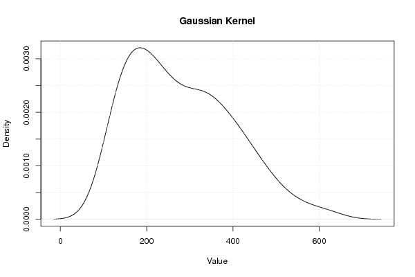
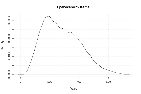
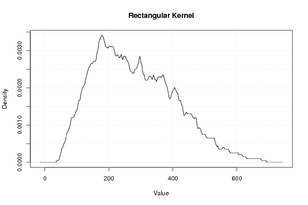
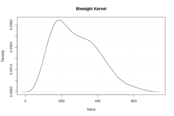
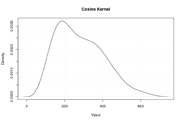
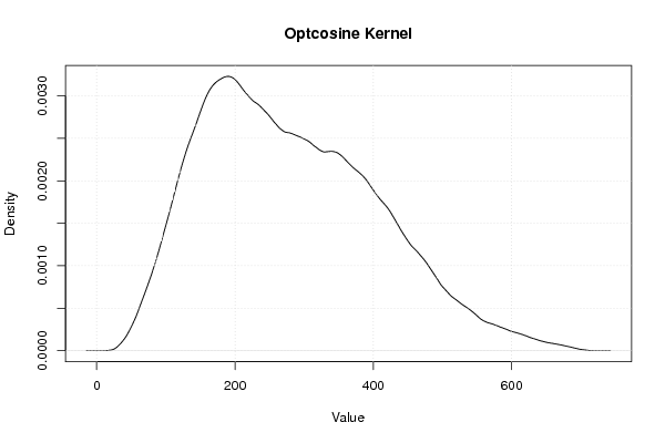
| Title produced by software | Kernel Density Estimation | ||||||||||||||||||||||||||||||||
| Date of computation | Wed, 30 Nov 2011 09:45:46 -0500 | ||||||||||||||||||||||||||||||||
| Cite this page as follows | Statistical Computations at FreeStatistics.org, Office for Research Development and Education, URL https://freestatistics.org/blog/index.php?v=date/2011/Nov/30/t1322664360mmythhebzwwxozu.htm/, Retrieved Tue, 08 Jul 2025 11:02:22 +0000 | ||||||||||||||||||||||||||||||||
| Statistical Computations at FreeStatistics.org, Office for Research Development and Education, URL https://freestatistics.org/blog/index.php?pk=148999, Retrieved Tue, 08 Jul 2025 11:02:22 +0000 | |||||||||||||||||||||||||||||||||
| QR Codes: | |||||||||||||||||||||||||||||||||
|
| |||||||||||||||||||||||||||||||||
| Original text written by user: | |||||||||||||||||||||||||||||||||
| IsPrivate? | No (this computation is public) | ||||||||||||||||||||||||||||||||
| User-defined keywords | |||||||||||||||||||||||||||||||||
| Estimated Impact | 206 | ||||||||||||||||||||||||||||||||
Tree of Dependent Computations | |||||||||||||||||||||||||||||||||
| Family? (F = Feedback message, R = changed R code, M = changed R Module, P = changed Parameters, D = changed Data) | |||||||||||||||||||||||||||||||||
| - [Kernel Density Estimation] [] [2011-11-30 14:45:46] [4cf172296f32adf71d8383c359dbb80f] [Current] - RM [Kernel Density Estimation] [] [2011-11-30 14:46:20] [f98f9dc58dd24d7896d4ecb781e1c75c] - RMP [Univariate Data Series] [] [2011-11-30 14:46:52] [f98f9dc58dd24d7896d4ecb781e1c75c] - RMP [Tukey lambda PPCC Plot] [] [2011-11-30 14:48:25] [f98f9dc58dd24d7896d4ecb781e1c75c] - RMPD [Pearson Correlation] [] [2011-11-30 14:49:33] [f98f9dc58dd24d7896d4ecb781e1c75c] - RMP [Bivariate Kernel Density Estimation] [] [2011-11-30 14:52:33] [f98f9dc58dd24d7896d4ecb781e1c75c] - RMPD [Blocked Bootstrap Plot - Central Tendency] [] [2011-11-30 14:53:39] [f98f9dc58dd24d7896d4ecb781e1c75c] | |||||||||||||||||||||||||||||||||
| Feedback Forum | |||||||||||||||||||||||||||||||||
Post a new message | |||||||||||||||||||||||||||||||||
Dataset | |||||||||||||||||||||||||||||||||
| Dataseries X: | |||||||||||||||||||||||||||||||||
113 119 133 130 122 136 149 149 137 120 105 119 116 127 142 136 126 150 171 171 159 134 115 141 146 151 179 164 173 179 200 200 185 163 147 167 172 181 194 182 184 219 231 243 210 192 173 195 197 197 237 236 230 244 265 273 238 212 181 202 205 189 236 228 235 265 303 294 260 230 204 230 243 234 268 270 271 316 365 348 313 275 238 279 285 278 318 314 319 375 414 406 356 307 272 307 316 302 357 349 356 423 466 468 405 348 306 337 341 319 363 349 364 436 492 506 405 360 311 338 361 343 407 397 421 473 549 560 464 408 363 406 418 392 420 462 473 536 623 607 509 462 391 433 | |||||||||||||||||||||||||||||||||
Tables (Output of Computation) | |||||||||||||||||||||||||||||||||
| |||||||||||||||||||||||||||||||||
Figures (Output of Computation) | |||||||||||||||||||||||||||||||||
Input Parameters & R Code | |||||||||||||||||||||||||||||||||
| Parameters (Session): | |||||||||||||||||||||||||||||||||
| par1 = 0 ; | |||||||||||||||||||||||||||||||||
| Parameters (R input): | |||||||||||||||||||||||||||||||||
| par1 = 0 ; | |||||||||||||||||||||||||||||||||
| R code (references can be found in the software module): | |||||||||||||||||||||||||||||||||
if (par1 == '0') bw <- 'nrd0' | |||||||||||||||||||||||||||||||||