Repository of Reproducible Computations

Free Statistics

of Irreproducible Research!

Author's title

Author

*Unverified author*

R Software Module

rwasp_autocorrelation.wasp

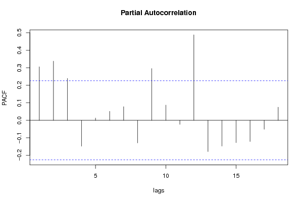
Title produced by software

(Partial) Autocorrelation Function

Date of computation

Tue, 29 Nov 2011 08:04:17 -0500

Cite this page as follows

Statistical Computations at FreeStatistics.org, Office for Research Development and Education, URL https://freestatistics.org/blog/index.php?v=date/2011/Nov/29/t1322571888lusda2nv4mk5d9f.htm/, Retrieved Thu, 25 Apr 2024 15:07:07 +0000

Statistical Computations at FreeStatistics.org, Office for Research Development and Education, URL https://freestatistics.org/blog/index.php?pk=148313, Retrieved Thu, 25 Apr 2024 15:07:07 +0000

QR Codes:

Paste this QR Code to cite your computation.

Original text written by user:

IsPrivate?

No (this computation is public)

User-defined keywords

Estimated Impact

103

Family? (F = Feedback message, R = changed R code, M = changed R Module, P = changed Parameters, D = changed Data)

F     [Univariate Data Series] [HPC Retail Sales] [2008-03-02 15:42:48] [74be16979710d4c4e7c6647856088456]
- RMPD  [Central Tendency] [Workshop 8, Robus...] [2010-11-28 19:41:12] [d946de7cca328fbcf207448a112523ab]
-         [Central Tendency] [Workshop 8, Centr...] [2010-11-29 20:08:54] [3635fb7041b1998c5a1332cf9de22bce]
- RMP       [(Partial) Autocorrelation Function] [Workshop 8 autoco...] [2010-11-30 11:00:00] [a9e130f95bad0a0597234e75c6380c5a]
- R  D          [(Partial) Autocorrelation Function] [WS8 - Mini-tutori...] [2011-11-29 13:04:17] [d41d8cd98f00b204e9800998ecf8427e] [Current]
-    D            [(Partial) Autocorrelation Function] [Paper Deel 2 - Da...] [2011-12-20 10:22:05] [95a4a8598e82ac3272c4dca488d0ba38] 

Feedback Forum

Post a new message

Dataseries X:

Download CSV

Histogram

Boxplots

Summary of computational transaction
Raw Input	view raw input (R code)
Raw Output	view raw output of R engine
Computing time	1 seconds
R Server	'Gwilym Jenkins' @ jenkins.wessa.net

\begin{tabular}{lllllllll}
\hline
Summary of computational transaction \tabularnewline
Raw Input & view raw input (R code)  \tabularnewline
Raw Output & view raw output of R engine  \tabularnewline
Computing time & 1 seconds \tabularnewline
R Server & 'Gwilym Jenkins' @ jenkins.wessa.net \tabularnewline
\hline
\end{tabular}
%Source: https://freestatistics.org/blog/index.php?pk=148313&T=0

[TABLE]
[ROW][C]Summary of computational transaction[/C][/ROW]
[ROW][C]Raw Input[/C][C]view raw input (R code) [/C][/ROW]
[ROW][C]Raw Output[/C][C]view raw output of R engine [/C][/ROW]
[ROW][C]Computing time[/C][C]1 seconds[/C][/ROW]
[ROW][C]R Server[/C][C]'Gwilym Jenkins' @ jenkins.wessa.net[/C][/ROW]
[/TABLE]
Source: https://freestatistics.org/blog/index.php?pk=148313&T=0

Globally Unique Identifier (entire table): ba.freestatistics.org/blog/index.php?pk=148313&T=0

As an alternative you can also use a QR Code:

The GUIDs for individual cells are displayed in the table below:

Summary of computational transaction
Raw Input	view raw input (R code)
Raw Output	view raw output of R engine
Computing time	1 seconds
R Server	'Gwilym Jenkins' @ jenkins.wessa.net

Autocorrelation Function
Time lag k	ACF(k)	T-STAT	P-value
1	0.305819	2.6485	0.004926
2	0.399873	3.463	0.000443
3	0.376736	3.2626	0.000832
4	0.122726	1.0628	0.145632
5	0.211704	1.8334	0.035354
6	0.151412	1.3113	0.096884
7	0.13703	1.1867	0.119543
8	0.039429	0.3415	0.366853
9	0.292297	2.5314	0.006728
10	0.162233	1.405	0.082079
11	0.162612	1.4083	0.081593
12	0.578733	5.012	2e-06
13	0.12317	1.0667	0.144768
14	0.273848	2.3716	0.010139
15	0.185348	1.6052	0.05633
16	-0.025095	-0.2173	0.41427
17	0.056483	0.4892	0.313079
18	0.043505	0.3768	0.353705

\begin{tabular}{lllllllll}
\hline
Autocorrelation Function \tabularnewline
Time lag k & ACF(k) & T-STAT & P-value \tabularnewline
1 & 0.305819 & 2.6485 & 0.004926 \tabularnewline
2 & 0.399873 & 3.463 & 0.000443 \tabularnewline
3 & 0.376736 & 3.2626 & 0.000832 \tabularnewline
4 & 0.122726 & 1.0628 & 0.145632 \tabularnewline
5 & 0.211704 & 1.8334 & 0.035354 \tabularnewline
6 & 0.151412 & 1.3113 & 0.096884 \tabularnewline
7 & 0.13703 & 1.1867 & 0.119543 \tabularnewline
8 & 0.039429 & 0.3415 & 0.366853 \tabularnewline
9 & 0.292297 & 2.5314 & 0.006728 \tabularnewline
10 & 0.162233 & 1.405 & 0.082079 \tabularnewline
11 & 0.162612 & 1.4083 & 0.081593 \tabularnewline
12 & 0.578733 & 5.012 & 2e-06 \tabularnewline
13 & 0.12317 & 1.0667 & 0.144768 \tabularnewline
14 & 0.273848 & 2.3716 & 0.010139 \tabularnewline
15 & 0.185348 & 1.6052 & 0.05633 \tabularnewline
16 & -0.025095 & -0.2173 & 0.41427 \tabularnewline
17 & 0.056483 & 0.4892 & 0.313079 \tabularnewline
18 & 0.043505 & 0.3768 & 0.353705 \tabularnewline
\hline
\end{tabular}
%Source: https://freestatistics.org/blog/index.php?pk=148313&T=1

[TABLE]
[ROW][C]Autocorrelation Function[/C][/ROW]
[ROW][C]Time lag k[/C][C]ACF(k)[/C][C]T-STAT[/C][C]P-value[/C][/ROW]
[ROW][C]1[/C][C]0.305819[/C][C]2.6485[/C][C]0.004926[/C][/ROW]
[ROW][C]2[/C][C]0.399873[/C][C]3.463[/C][C]0.000443[/C][/ROW]
[ROW][C]3[/C][C]0.376736[/C][C]3.2626[/C][C]0.000832[/C][/ROW]
[ROW][C]4[/C][C]0.122726[/C][C]1.0628[/C][C]0.145632[/C][/ROW]
[ROW][C]5[/C][C]0.211704[/C][C]1.8334[/C][C]0.035354[/C][/ROW]
[ROW][C]6[/C][C]0.151412[/C][C]1.3113[/C][C]0.096884[/C][/ROW]
[ROW][C]7[/C][C]0.13703[/C][C]1.1867[/C][C]0.119543[/C][/ROW]
[ROW][C]8[/C][C]0.039429[/C][C]0.3415[/C][C]0.366853[/C][/ROW]
[ROW][C]9[/C][C]0.292297[/C][C]2.5314[/C][C]0.006728[/C][/ROW]
[ROW][C]10[/C][C]0.162233[/C][C]1.405[/C][C]0.082079[/C][/ROW]
[ROW][C]11[/C][C]0.162612[/C][C]1.4083[/C][C]0.081593[/C][/ROW]
[ROW][C]12[/C][C]0.578733[/C][C]5.012[/C][C]2e-06[/C][/ROW]
[ROW][C]13[/C][C]0.12317[/C][C]1.0667[/C][C]0.144768[/C][/ROW]
[ROW][C]14[/C][C]0.273848[/C][C]2.3716[/C][C]0.010139[/C][/ROW]
[ROW][C]15[/C][C]0.185348[/C][C]1.6052[/C][C]0.05633[/C][/ROW]
[ROW][C]16[/C][C]-0.025095[/C][C]-0.2173[/C][C]0.41427[/C][/ROW]
[ROW][C]17[/C][C]0.056483[/C][C]0.4892[/C][C]0.313079[/C][/ROW]
[ROW][C]18[/C][C]0.043505[/C][C]0.3768[/C][C]0.353705[/C][/ROW]
[/TABLE]
Source: https://freestatistics.org/blog/index.php?pk=148313&T=1

Globally Unique Identifier (entire table): ba.freestatistics.org/blog/index.php?pk=148313&T=1

As an alternative you can also use a QR Code:

The GUIDs for individual cells are displayed in the table below:

Autocorrelation Function
Time lag k	ACF(k)	T-STAT	P-value
1	0.305819	2.6485	0.004926
2	0.399873	3.463	0.000443
3	0.376736	3.2626	0.000832
4	0.122726	1.0628	0.145632
5	0.211704	1.8334	0.035354
6	0.151412	1.3113	0.096884
7	0.13703	1.1867	0.119543
8	0.039429	0.3415	0.366853
9	0.292297	2.5314	0.006728
10	0.162233	1.405	0.082079
11	0.162612	1.4083	0.081593
12	0.578733	5.012	2e-06
13	0.12317	1.0667	0.144768
14	0.273848	2.3716	0.010139
15	0.185348	1.6052	0.05633
16	-0.025095	-0.2173	0.41427
17	0.056483	0.4892	0.313079
18	0.043505	0.3768	0.353705

Partial Autocorrelation Function
Time lag k	PACF(k)	T-STAT	P-value
1	0.305819	2.6485	0.004926
2	0.337955	2.9268	0.002265
3	0.239646	2.0754	0.020689
4	-0.14807	-1.2823	0.10184
5	0.012857	0.1113	0.45582
6	0.051396	0.4451	0.328763
7	0.078059	0.676	0.250558
8	-0.12924	-1.1193	0.133301
9	0.295804	2.5617	0.006211
10	0.086951	0.753	0.226898
11	-0.023225	-0.2011	0.420569
12	0.488393	4.2296	3.3e-05
13	-0.178637	-1.547	0.063031
14	-0.147488	-1.2773	0.102721
15	-0.127635	-1.1054	0.13627
16	-0.121525	-1.0524	0.14799
17	-0.05138	-0.445	0.328814
18	0.075129	0.6506	0.258634

\begin{tabular}{lllllllll}
\hline
Partial Autocorrelation Function \tabularnewline
Time lag k & PACF(k) & T-STAT & P-value \tabularnewline
1 & 0.305819 & 2.6485 & 0.004926 \tabularnewline
2 & 0.337955 & 2.9268 & 0.002265 \tabularnewline
3 & 0.239646 & 2.0754 & 0.020689 \tabularnewline
4 & -0.14807 & -1.2823 & 0.10184 \tabularnewline
5 & 0.012857 & 0.1113 & 0.45582 \tabularnewline
6 & 0.051396 & 0.4451 & 0.328763 \tabularnewline
7 & 0.078059 & 0.676 & 0.250558 \tabularnewline
8 & -0.12924 & -1.1193 & 0.133301 \tabularnewline
9 & 0.295804 & 2.5617 & 0.006211 \tabularnewline
10 & 0.086951 & 0.753 & 0.226898 \tabularnewline
11 & -0.023225 & -0.2011 & 0.420569 \tabularnewline
12 & 0.488393 & 4.2296 & 3.3e-05 \tabularnewline
13 & -0.178637 & -1.547 & 0.063031 \tabularnewline
14 & -0.147488 & -1.2773 & 0.102721 \tabularnewline
15 & -0.127635 & -1.1054 & 0.13627 \tabularnewline
16 & -0.121525 & -1.0524 & 0.14799 \tabularnewline
17 & -0.05138 & -0.445 & 0.328814 \tabularnewline
18 & 0.075129 & 0.6506 & 0.258634 \tabularnewline
\hline
\end{tabular}
%Source: https://freestatistics.org/blog/index.php?pk=148313&T=2

[TABLE]
[ROW][C]Partial Autocorrelation Function[/C][/ROW]
[ROW][C]Time lag k[/C][C]PACF(k)[/C][C]T-STAT[/C][C]P-value[/C][/ROW]
[ROW][C]1[/C][C]0.305819[/C][C]2.6485[/C][C]0.004926[/C][/ROW]
[ROW][C]2[/C][C]0.337955[/C][C]2.9268[/C][C]0.002265[/C][/ROW]
[ROW][C]3[/C][C]0.239646[/C][C]2.0754[/C][C]0.020689[/C][/ROW]
[ROW][C]4[/C][C]-0.14807[/C][C]-1.2823[/C][C]0.10184[/C][/ROW]
[ROW][C]5[/C][C]0.012857[/C][C]0.1113[/C][C]0.45582[/C][/ROW]
[ROW][C]6[/C][C]0.051396[/C][C]0.4451[/C][C]0.328763[/C][/ROW]
[ROW][C]7[/C][C]0.078059[/C][C]0.676[/C][C]0.250558[/C][/ROW]
[ROW][C]8[/C][C]-0.12924[/C][C]-1.1193[/C][C]0.133301[/C][/ROW]
[ROW][C]9[/C][C]0.295804[/C][C]2.5617[/C][C]0.006211[/C][/ROW]
[ROW][C]10[/C][C]0.086951[/C][C]0.753[/C][C]0.226898[/C][/ROW]
[ROW][C]11[/C][C]-0.023225[/C][C]-0.2011[/C][C]0.420569[/C][/ROW]
[ROW][C]12[/C][C]0.488393[/C][C]4.2296[/C][C]3.3e-05[/C][/ROW]
[ROW][C]13[/C][C]-0.178637[/C][C]-1.547[/C][C]0.063031[/C][/ROW]
[ROW][C]14[/C][C]-0.147488[/C][C]-1.2773[/C][C]0.102721[/C][/ROW]
[ROW][C]15[/C][C]-0.127635[/C][C]-1.1054[/C][C]0.13627[/C][/ROW]
[ROW][C]16[/C][C]-0.121525[/C][C]-1.0524[/C][C]0.14799[/C][/ROW]
[ROW][C]17[/C][C]-0.05138[/C][C]-0.445[/C][C]0.328814[/C][/ROW]
[ROW][C]18[/C][C]0.075129[/C][C]0.6506[/C][C]0.258634[/C][/ROW]
[/TABLE]
Source: https://freestatistics.org/blog/index.php?pk=148313&T=2

Globally Unique Identifier (entire table): ba.freestatistics.org/blog/index.php?pk=148313&T=2

As an alternative you can also use a QR Code:

The GUIDs for individual cells are displayed in the table below:

Partial Autocorrelation Function
Time lag k	PACF(k)	T-STAT	P-value
1	0.305819	2.6485	0.004926
2	0.337955	2.9268	0.002265
3	0.239646	2.0754	0.020689
4	-0.14807	-1.2823	0.10184
5	0.012857	0.1113	0.45582
6	0.051396	0.4451	0.328763
7	0.078059	0.676	0.250558
8	-0.12924	-1.1193	0.133301
9	0.295804	2.5617	0.006211
10	0.086951	0.753	0.226898
11	-0.023225	-0.2011	0.420569
12	0.488393	4.2296	3.3e-05
13	-0.178637	-1.547	0.063031
14	-0.147488	-1.2773	0.102721
15	-0.127635	-1.1054	0.13627
16	-0.121525	-1.0524	0.14799
17	-0.05138	-0.445	0.328814
18	0.075129	0.6506	0.258634

Figure 1

PNG link

Postscript link

PDF link

Figure 2

PNG link

Postscript link

PDF link

Parameters (Session):

par1 = Default ; par2 = 1 ; par3 = 0 ; par4 = 0 ; par5 = 12 ; par6 = White Noise ; par7 = 0.95 ;

Parameters (R input):

par1 = Default ; par2 = 1 ; par3 = 0 ; par4 = 0 ; par5 = 12 ; par6 = White Noise ; par7 = 0.95 ; par8 = ;

R code (references can be found in the software module):

if (par1 == 'Default') {
par1 = 10*log10(length(x))
} else {
par1 <- as.numeric(par1)
}
par2 <- as.numeric(par2)
par3 <- as.numeric(par3)
par4 <- as.numeric(par4)
par5 <- as.numeric(par5)
if (par6 == 'White Noise') par6 <- 'white' else par6 <- 'ma'
par7 <- as.numeric(par7)
if (par2 == 0) {
x <- log(x)
} else {
x <- (x ^ par2 - 1) / par2
}
if (par3 > 0) x <- diff(x,lag=1,difference=par3)
if (par4 > 0) x <- diff(x,lag=par5,difference=par4)
bitmap(file='pic1.png')
racf <- acf(x, par1, main='Autocorrelation', xlab='time lag', ylab='ACF', ci.type=par6, ci=par7, sub=paste('(lambda=',par2,', d=',par3,', D=',par4,', CI=', par7, ', CI type=',par6,')',sep=''))
dev.off()
bitmap(file='pic2.png')
rpacf <- pacf(x,par1,main='Partial Autocorrelation',xlab='lags',ylab='PACF')
dev.off()
(myacf <- c(racf$acf))
(mypacf <- c(rpacf$acf))
lengthx <- length(x)
sqrtn <- sqrt(lengthx)
load(file='createtable')
a<-table.start()
a<-table.row.start(a)
a<-table.element(a,'Autocorrelation Function',4,TRUE)
a<-table.row.end(a)
a<-table.row.start(a)
a<-table.element(a,'Time lag k',header=TRUE)
a<-table.element(a,hyperlink('basics.htm','ACF(k)','click here for more information about the Autocorrelation Function'),header=TRUE)
a<-table.element(a,'T-STAT',header=TRUE)
a<-table.element(a,'P-value',header=TRUE)
a<-table.row.end(a)
for (i in 2:(par1+1)) {
a<-table.row.start(a)
a<-table.element(a,i-1,header=TRUE)
a<-table.element(a,round(myacf[i],6))
mytstat <- myacf[i]*sqrtn
a<-table.element(a,round(mytstat,4))
a<-table.element(a,round(1-pt(abs(mytstat),lengthx),6))
a<-table.row.end(a)
}
a<-table.end(a)
table.save(a,file='mytable.tab')
a<-table.start()
a<-table.row.start(a)
a<-table.element(a,'Partial Autocorrelation Function',4,TRUE)
a<-table.row.end(a)
a<-table.row.start(a)
a<-table.element(a,'Time lag k',header=TRUE)
a<-table.element(a,hyperlink('basics.htm','PACF(k)','click here for more information about the Partial Autocorrelation Function'),header=TRUE)
a<-table.element(a,'T-STAT',header=TRUE)
a<-table.element(a,'P-value',header=TRUE)
a<-table.row.end(a)
for (i in 1:par1) {
a<-table.row.start(a)
a<-table.element(a,i,header=TRUE)
a<-table.element(a,round(mypacf[i],6))
mytstat <- mypacf[i]*sqrtn
a<-table.element(a,round(mytstat,4))
a<-table.element(a,round(1-pt(abs(mytstat),lengthx),6))
a<-table.row.end(a)
}
a<-table.end(a)
table.save(a,file='mytable1.tab')

Free Statistics

Description of Statistical Computation

Tree of Dependent Computations

Dataset

Tables (Output of Computation)

Figures (Output of Computation)

Input Parameters & R Code