Repository of Reproducible Computations

Free Statistics

of Irreproducible Research!

Author's title

Author

*The author of this computation has been verified*

R Software Module

rwasp_percentiles.wasp

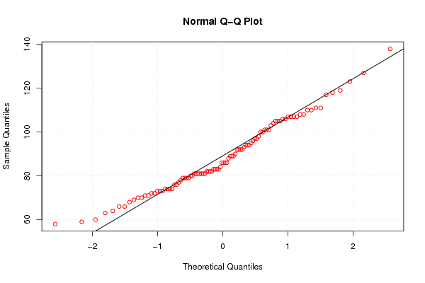
Title produced by software

Percentiles

Date of computation

Tue, 29 Nov 2011 07:35:38 -0500

Cite this page as follows

Statistical Computations at FreeStatistics.org, Office for Research Development and Education, URL https://freestatistics.org/blog/index.php?v=date/2011/Nov/29/t1322570160limftkzpvdw7ftp.htm/, Retrieved Fri, 26 Apr 2024 21:51:26 +0000

Statistical Computations at FreeStatistics.org, Office for Research Development and Education, URL https://freestatistics.org/blog/index.php?pk=148260, Retrieved Fri, 26 Apr 2024 21:51:26 +0000

QR Codes:

Paste this QR Code to cite your computation.

Original text written by user:

IsPrivate?

No (this computation is public)

User-defined keywords

percentielen

Estimated Impact

125

Family? (F = Feedback message, R = changed R code, M = changed R Module, P = changed Parameters, D = changed Data)

-     [Stem-and-leaf Plot] [Paper] [2011-11-29 10:42:53] [227e53f633d125e3e89f625705633e7f]
- RMPD    [Percentiles] [Paper] [2011-11-29 12:35:38] [065e524ef27b3ebe8baf73e00eb8c266] [Current]
- RM        [Harrell-Davis Quantiles] [Paper] [2011-11-29 12:41:15] [227e53f633d125e3e89f625705633e7f] 
- RMP       [Maximum-likelihood Fitting - Normal Distribution] [Paper] [2011-12-06 09:27:01] [227e53f633d125e3e89f625705633e7f] 
- RM        [Tukey lambda PPCC Plot] [paper] [2011-12-06 09:31:08] [227e53f633d125e3e89f625705633e7f] 
-    D      [Percentiles] [] [2011-12-16 14:26:29] [a9dc51245fb8ca00f931d89893d090c8] 
- RMP       [Notched Boxplots] [Paper] [2011-12-19 17:01:19] [227e53f633d125e3e89f625705633e7f] 
- RMPD      [Paired and Unpaired Two Samples Tests about the Mean] [Paper] [2011-12-19 18:27:52] [227e53f633d125e3e89f625705633e7f] 
- R PD        [Paired and Unpaired Two Samples Tests about the Mean] [Paper] [2011-12-19 18:38:55] [227e53f633d125e3e89f625705633e7f] 
- R  D        [Paired and Unpaired Two Samples Tests about the Mean] [Paper] [2011-12-19 18:40:26] [227e53f633d125e3e89f625705633e7f] 

Feedback Forum

Post a new message

Dataseries X:

Download CSV

Histogram

Boxplots

Summary of computational transaction
Raw Input	view raw input (R code)
Raw Output	view raw output of R engine
Computing time	0 seconds
R Server	'Gwilym Jenkins' @ jenkins.wessa.net

\begin{tabular}{lllllllll}
\hline
Summary of computational transaction \tabularnewline
Raw Input & view raw input (R code)  \tabularnewline
Raw Output & view raw output of R engine  \tabularnewline
Computing time & 0 seconds \tabularnewline
R Server & 'Gwilym Jenkins' @ jenkins.wessa.net \tabularnewline
\hline
\end{tabular}
%Source: https://freestatistics.org/blog/index.php?pk=148260&T=0

[TABLE]
[ROW][C]Summary of computational transaction[/C][/ROW]
[ROW][C]Raw Input[/C][C]view raw input (R code) [/C][/ROW]
[ROW][C]Raw Output[/C][C]view raw output of R engine [/C][/ROW]
[ROW][C]Computing time[/C][C]0 seconds[/C][/ROW]
[ROW][C]R Server[/C][C]'Gwilym Jenkins' @ jenkins.wessa.net[/C][/ROW]
[/TABLE]
Source: https://freestatistics.org/blog/index.php?pk=148260&T=0

Globally Unique Identifier (entire table): ba.freestatistics.org/blog/index.php?pk=148260&T=0

As an alternative you can also use a QR Code:

The GUIDs for individual cells are displayed in the table below:

Summary of computational transaction
Raw Input	view raw input (R code)
Raw Output	view raw output of R engine
Computing time	0 seconds
R Server	'Gwilym Jenkins' @ jenkins.wessa.net

Percentiles - Ungrouped Data
p	Weighted Average at Xnp	Weighted Average at X(n+1)p	Empirical Distribution Function	Empirical Distribution Function - Averaging	Empirical Distribution Function - Interpolation	Closest Observation	True Basic - Statistics Graphics Toolkit	MS Excel (old versions)
0.02	58.96	58.98	59	59	59.94	59	58.02	59
0.04	62.76	62.88	63	63	63.88	63	60.12	63
0.06	65.76	65.88	66	66	66	66	64.12	66
0.08	67.68	67.84	68	68	68.76	68	66.16	68
0.1	69.8	69.9	70	70	70	70	69.1	70
0.12	70.76	70.88	71	71	71	71	70.12	71
0.14	71.72	71.86	72	72	72	72	71.14	72
0.16	72.68	72.84	73	73	73	73	72.16	73
0.18	73	73	73	73	73.46	73	73	73
0.2	74	74	74	74	74	74	74	74
0.22	74	74	74	74	74.68	74	74	74
0.24	76	76	76	76	76.28	76	76	76
0.26	77.48	77.74	78	78	78.22	77	77.26	78
0.28	79	79	79	79	79	79	79	79
0.3	79	79	79	79	79.1	79	79	79
0.32	80	80	80	80	80.04	80	80	80
0.34	81	81	81	81	81	81	81	81
0.36	81	81	81	81	81	81	81	81
0.38	81	81	81	81	81	81	81	81
0.4	81.2	81.6	82	82	81.8	81	81.4	82
0.42	82	82	82	82	82	82	82	82
0.44	82.12	82.56	83	83	82.68	82	82.44	83
0.46	83	83	83	83	83	83	83	83
0.48	83.04	83.52	84	84	83.56	83	83.48	84
0.5	86	86	86	86	86	86	86	86
0.52	86	86	86	86	86	86	86	86
0.54	87.84	88.46	88	88	88.38	88	88.54	88
0.56	89	89	89	89	89	89	89	89
0.58	89.84	90.84	90	90	90.52	90	91.16	90
0.6	92	92	92	92	92	92	92	92
0.62	92	92.38	92	92	92.14	92	92.62	92
0.64	93.72	94	94	94	94	94	94	94
0.66	94	94.34	94	94	94.02	94	94.66	94
0.68	95.64	96.32	96	96	95.96	96	96.68	96
0.7	97	97.3	97	97	97	97	97.7	97
0.72	99.12	100	100	100	99.68	100	100	100
0.74	100.52	101	101	101	100.78	101	101	101
0.76	101	101.48	101	101	101	101	102.52	101
0.78	103.44	104.22	104	104	103.66	103	104.78	104
0.8	105	105	105	105	105	105	105	105
0.82	105.36	106	106	106	105.54	105	106	106
0.84	106.32	107	107	107	106.48	106	107	107
0.86	107	107	107	107	107	107	107	107
0.88	107.24	108	108	108	107.36	107	108	108
0.9	108.4	110	110	110	108.6	108	110	110
0.92	110.16	111	111	111	110.24	110	111	111
0.94	111.72	117.06	117	117	112.08	111	117.94	117
0.96	118.08	119.16	119	119	118.12	118	122.84	119
0.98	123.16	127.22	127	127	123.24	123	137.78	127

\begin{tabular}{lllllllll}
\hline
Percentiles - Ungrouped Data \tabularnewline
p & Weighted Average at Xnp & Weighted Average at X(n+1)p & Empirical Distribution Function & Empirical Distribution Function - Averaging & Empirical Distribution Function - Interpolation & Closest Observation & True Basic - Statistics Graphics Toolkit & MS Excel (old versions) \tabularnewline
0.02 & 58.96 & 58.98 & 59 & 59 & 59.94 & 59 & 58.02 & 59 \tabularnewline
0.04 & 62.76 & 62.88 & 63 & 63 & 63.88 & 63 & 60.12 & 63 \tabularnewline
0.06 & 65.76 & 65.88 & 66 & 66 & 66 & 66 & 64.12 & 66 \tabularnewline
0.08 & 67.68 & 67.84 & 68 & 68 & 68.76 & 68 & 66.16 & 68 \tabularnewline
0.1 & 69.8 & 69.9 & 70 & 70 & 70 & 70 & 69.1 & 70 \tabularnewline
0.12 & 70.76 & 70.88 & 71 & 71 & 71 & 71 & 70.12 & 71 \tabularnewline
0.14 & 71.72 & 71.86 & 72 & 72 & 72 & 72 & 71.14 & 72 \tabularnewline
0.16 & 72.68 & 72.84 & 73 & 73 & 73 & 73 & 72.16 & 73 \tabularnewline
0.18 & 73 & 73 & 73 & 73 & 73.46 & 73 & 73 & 73 \tabularnewline
0.2 & 74 & 74 & 74 & 74 & 74 & 74 & 74 & 74 \tabularnewline
0.22 & 74 & 74 & 74 & 74 & 74.68 & 74 & 74 & 74 \tabularnewline
0.24 & 76 & 76 & 76 & 76 & 76.28 & 76 & 76 & 76 \tabularnewline
0.26 & 77.48 & 77.74 & 78 & 78 & 78.22 & 77 & 77.26 & 78 \tabularnewline
0.28 & 79 & 79 & 79 & 79 & 79 & 79 & 79 & 79 \tabularnewline
0.3 & 79 & 79 & 79 & 79 & 79.1 & 79 & 79 & 79 \tabularnewline
0.32 & 80 & 80 & 80 & 80 & 80.04 & 80 & 80 & 80 \tabularnewline
0.34 & 81 & 81 & 81 & 81 & 81 & 81 & 81 & 81 \tabularnewline
0.36 & 81 & 81 & 81 & 81 & 81 & 81 & 81 & 81 \tabularnewline
0.38 & 81 & 81 & 81 & 81 & 81 & 81 & 81 & 81 \tabularnewline
0.4 & 81.2 & 81.6 & 82 & 82 & 81.8 & 81 & 81.4 & 82 \tabularnewline
0.42 & 82 & 82 & 82 & 82 & 82 & 82 & 82 & 82 \tabularnewline
0.44 & 82.12 & 82.56 & 83 & 83 & 82.68 & 82 & 82.44 & 83 \tabularnewline
0.46 & 83 & 83 & 83 & 83 & 83 & 83 & 83 & 83 \tabularnewline
0.48 & 83.04 & 83.52 & 84 & 84 & 83.56 & 83 & 83.48 & 84 \tabularnewline
0.5 & 86 & 86 & 86 & 86 & 86 & 86 & 86 & 86 \tabularnewline
0.52 & 86 & 86 & 86 & 86 & 86 & 86 & 86 & 86 \tabularnewline
0.54 & 87.84 & 88.46 & 88 & 88 & 88.38 & 88 & 88.54 & 88 \tabularnewline
0.56 & 89 & 89 & 89 & 89 & 89 & 89 & 89 & 89 \tabularnewline
0.58 & 89.84 & 90.84 & 90 & 90 & 90.52 & 90 & 91.16 & 90 \tabularnewline
0.6 & 92 & 92 & 92 & 92 & 92 & 92 & 92 & 92 \tabularnewline
0.62 & 92 & 92.38 & 92 & 92 & 92.14 & 92 & 92.62 & 92 \tabularnewline
0.64 & 93.72 & 94 & 94 & 94 & 94 & 94 & 94 & 94 \tabularnewline
0.66 & 94 & 94.34 & 94 & 94 & 94.02 & 94 & 94.66 & 94 \tabularnewline
0.68 & 95.64 & 96.32 & 96 & 96 & 95.96 & 96 & 96.68 & 96 \tabularnewline
0.7 & 97 & 97.3 & 97 & 97 & 97 & 97 & 97.7 & 97 \tabularnewline
0.72 & 99.12 & 100 & 100 & 100 & 99.68 & 100 & 100 & 100 \tabularnewline
0.74 & 100.52 & 101 & 101 & 101 & 100.78 & 101 & 101 & 101 \tabularnewline
0.76 & 101 & 101.48 & 101 & 101 & 101 & 101 & 102.52 & 101 \tabularnewline
0.78 & 103.44 & 104.22 & 104 & 104 & 103.66 & 103 & 104.78 & 104 \tabularnewline
0.8 & 105 & 105 & 105 & 105 & 105 & 105 & 105 & 105 \tabularnewline
0.82 & 105.36 & 106 & 106 & 106 & 105.54 & 105 & 106 & 106 \tabularnewline
0.84 & 106.32 & 107 & 107 & 107 & 106.48 & 106 & 107 & 107 \tabularnewline
0.86 & 107 & 107 & 107 & 107 & 107 & 107 & 107 & 107 \tabularnewline
0.88 & 107.24 & 108 & 108 & 108 & 107.36 & 107 & 108 & 108 \tabularnewline
0.9 & 108.4 & 110 & 110 & 110 & 108.6 & 108 & 110 & 110 \tabularnewline
0.92 & 110.16 & 111 & 111 & 111 & 110.24 & 110 & 111 & 111 \tabularnewline
0.94 & 111.72 & 117.06 & 117 & 117 & 112.08 & 111 & 117.94 & 117 \tabularnewline
0.96 & 118.08 & 119.16 & 119 & 119 & 118.12 & 118 & 122.84 & 119 \tabularnewline
0.98 & 123.16 & 127.22 & 127 & 127 & 123.24 & 123 & 137.78 & 127 \tabularnewline
\hline
\end{tabular}
%Source: https://freestatistics.org/blog/index.php?pk=148260&T=1

[TABLE]
[ROW][C]Percentiles - Ungrouped Data[/C][/ROW]
[ROW][C]p[/C][C]Weighted Average at Xnp[/C][C]Weighted Average at X(n+1)p[/C][C]Empirical Distribution Function[/C][C]Empirical Distribution Function - Averaging[/C][C]Empirical Distribution Function - Interpolation[/C][C]Closest Observation[/C][C]True Basic - Statistics Graphics Toolkit[/C][C]MS Excel (old versions)[/C][/ROW]
[ROW][C]0.02[/C][C]58.96[/C][C]58.98[/C][C]59[/C][C]59[/C][C]59.94[/C][C]59[/C][C]58.02[/C][C]59[/C][/ROW]
[ROW][C]0.04[/C][C]62.76[/C][C]62.88[/C][C]63[/C][C]63[/C][C]63.88[/C][C]63[/C][C]60.12[/C][C]63[/C][/ROW]
[ROW][C]0.06[/C][C]65.76[/C][C]65.88[/C][C]66[/C][C]66[/C][C]66[/C][C]66[/C][C]64.12[/C][C]66[/C][/ROW]
[ROW][C]0.08[/C][C]67.68[/C][C]67.84[/C][C]68[/C][C]68[/C][C]68.76[/C][C]68[/C][C]66.16[/C][C]68[/C][/ROW]
[ROW][C]0.1[/C][C]69.8[/C][C]69.9[/C][C]70[/C][C]70[/C][C]70[/C][C]70[/C][C]69.1[/C][C]70[/C][/ROW]
[ROW][C]0.12[/C][C]70.76[/C][C]70.88[/C][C]71[/C][C]71[/C][C]71[/C][C]71[/C][C]70.12[/C][C]71[/C][/ROW]
[ROW][C]0.14[/C][C]71.72[/C][C]71.86[/C][C]72[/C][C]72[/C][C]72[/C][C]72[/C][C]71.14[/C][C]72[/C][/ROW]
[ROW][C]0.16[/C][C]72.68[/C][C]72.84[/C][C]73[/C][C]73[/C][C]73[/C][C]73[/C][C]72.16[/C][C]73[/C][/ROW]
[ROW][C]0.18[/C][C]73[/C][C]73[/C][C]73[/C][C]73[/C][C]73.46[/C][C]73[/C][C]73[/C][C]73[/C][/ROW]
[ROW][C]0.2[/C][C]74[/C][C]74[/C][C]74[/C][C]74[/C][C]74[/C][C]74[/C][C]74[/C][C]74[/C][/ROW]
[ROW][C]0.22[/C][C]74[/C][C]74[/C][C]74[/C][C]74[/C][C]74.68[/C][C]74[/C][C]74[/C][C]74[/C][/ROW]
[ROW][C]0.24[/C][C]76[/C][C]76[/C][C]76[/C][C]76[/C][C]76.28[/C][C]76[/C][C]76[/C][C]76[/C][/ROW]
[ROW][C]0.26[/C][C]77.48[/C][C]77.74[/C][C]78[/C][C]78[/C][C]78.22[/C][C]77[/C][C]77.26[/C][C]78[/C][/ROW]
[ROW][C]0.28[/C][C]79[/C][C]79[/C][C]79[/C][C]79[/C][C]79[/C][C]79[/C][C]79[/C][C]79[/C][/ROW]
[ROW][C]0.3[/C][C]79[/C][C]79[/C][C]79[/C][C]79[/C][C]79.1[/C][C]79[/C][C]79[/C][C]79[/C][/ROW]
[ROW][C]0.32[/C][C]80[/C][C]80[/C][C]80[/C][C]80[/C][C]80.04[/C][C]80[/C][C]80[/C][C]80[/C][/ROW]
[ROW][C]0.34[/C][C]81[/C][C]81[/C][C]81[/C][C]81[/C][C]81[/C][C]81[/C][C]81[/C][C]81[/C][/ROW]
[ROW][C]0.36[/C][C]81[/C][C]81[/C][C]81[/C][C]81[/C][C]81[/C][C]81[/C][C]81[/C][C]81[/C][/ROW]
[ROW][C]0.38[/C][C]81[/C][C]81[/C][C]81[/C][C]81[/C][C]81[/C][C]81[/C][C]81[/C][C]81[/C][/ROW]
[ROW][C]0.4[/C][C]81.2[/C][C]81.6[/C][C]82[/C][C]82[/C][C]81.8[/C][C]81[/C][C]81.4[/C][C]82[/C][/ROW]
[ROW][C]0.42[/C][C]82[/C][C]82[/C][C]82[/C][C]82[/C][C]82[/C][C]82[/C][C]82[/C][C]82[/C][/ROW]
[ROW][C]0.44[/C][C]82.12[/C][C]82.56[/C][C]83[/C][C]83[/C][C]82.68[/C][C]82[/C][C]82.44[/C][C]83[/C][/ROW]
[ROW][C]0.46[/C][C]83[/C][C]83[/C][C]83[/C][C]83[/C][C]83[/C][C]83[/C][C]83[/C][C]83[/C][/ROW]
[ROW][C]0.48[/C][C]83.04[/C][C]83.52[/C][C]84[/C][C]84[/C][C]83.56[/C][C]83[/C][C]83.48[/C][C]84[/C][/ROW]
[ROW][C]0.5[/C][C]86[/C][C]86[/C][C]86[/C][C]86[/C][C]86[/C][C]86[/C][C]86[/C][C]86[/C][/ROW]
[ROW][C]0.52[/C][C]86[/C][C]86[/C][C]86[/C][C]86[/C][C]86[/C][C]86[/C][C]86[/C][C]86[/C][/ROW]
[ROW][C]0.54[/C][C]87.84[/C][C]88.46[/C][C]88[/C][C]88[/C][C]88.38[/C][C]88[/C][C]88.54[/C][C]88[/C][/ROW]
[ROW][C]0.56[/C][C]89[/C][C]89[/C][C]89[/C][C]89[/C][C]89[/C][C]89[/C][C]89[/C][C]89[/C][/ROW]
[ROW][C]0.58[/C][C]89.84[/C][C]90.84[/C][C]90[/C][C]90[/C][C]90.52[/C][C]90[/C][C]91.16[/C][C]90[/C][/ROW]
[ROW][C]0.6[/C][C]92[/C][C]92[/C][C]92[/C][C]92[/C][C]92[/C][C]92[/C][C]92[/C][C]92[/C][/ROW]
[ROW][C]0.62[/C][C]92[/C][C]92.38[/C][C]92[/C][C]92[/C][C]92.14[/C][C]92[/C][C]92.62[/C][C]92[/C][/ROW]
[ROW][C]0.64[/C][C]93.72[/C][C]94[/C][C]94[/C][C]94[/C][C]94[/C][C]94[/C][C]94[/C][C]94[/C][/ROW]
[ROW][C]0.66[/C][C]94[/C][C]94.34[/C][C]94[/C][C]94[/C][C]94.02[/C][C]94[/C][C]94.66[/C][C]94[/C][/ROW]
[ROW][C]0.68[/C][C]95.64[/C][C]96.32[/C][C]96[/C][C]96[/C][C]95.96[/C][C]96[/C][C]96.68[/C][C]96[/C][/ROW]
[ROW][C]0.7[/C][C]97[/C][C]97.3[/C][C]97[/C][C]97[/C][C]97[/C][C]97[/C][C]97.7[/C][C]97[/C][/ROW]
[ROW][C]0.72[/C][C]99.12[/C][C]100[/C][C]100[/C][C]100[/C][C]99.68[/C][C]100[/C][C]100[/C][C]100[/C][/ROW]
[ROW][C]0.74[/C][C]100.52[/C][C]101[/C][C]101[/C][C]101[/C][C]100.78[/C][C]101[/C][C]101[/C][C]101[/C][/ROW]
[ROW][C]0.76[/C][C]101[/C][C]101.48[/C][C]101[/C][C]101[/C][C]101[/C][C]101[/C][C]102.52[/C][C]101[/C][/ROW]
[ROW][C]0.78[/C][C]103.44[/C][C]104.22[/C][C]104[/C][C]104[/C][C]103.66[/C][C]103[/C][C]104.78[/C][C]104[/C][/ROW]
[ROW][C]0.8[/C][C]105[/C][C]105[/C][C]105[/C][C]105[/C][C]105[/C][C]105[/C][C]105[/C][C]105[/C][/ROW]
[ROW][C]0.82[/C][C]105.36[/C][C]106[/C][C]106[/C][C]106[/C][C]105.54[/C][C]105[/C][C]106[/C][C]106[/C][/ROW]
[ROW][C]0.84[/C][C]106.32[/C][C]107[/C][C]107[/C][C]107[/C][C]106.48[/C][C]106[/C][C]107[/C][C]107[/C][/ROW]
[ROW][C]0.86[/C][C]107[/C][C]107[/C][C]107[/C][C]107[/C][C]107[/C][C]107[/C][C]107[/C][C]107[/C][/ROW]
[ROW][C]0.88[/C][C]107.24[/C][C]108[/C][C]108[/C][C]108[/C][C]107.36[/C][C]107[/C][C]108[/C][C]108[/C][/ROW]
[ROW][C]0.9[/C][C]108.4[/C][C]110[/C][C]110[/C][C]110[/C][C]108.6[/C][C]108[/C][C]110[/C][C]110[/C][/ROW]
[ROW][C]0.92[/C][C]110.16[/C][C]111[/C][C]111[/C][C]111[/C][C]110.24[/C][C]110[/C][C]111[/C][C]111[/C][/ROW]
[ROW][C]0.94[/C][C]111.72[/C][C]117.06[/C][C]117[/C][C]117[/C][C]112.08[/C][C]111[/C][C]117.94[/C][C]117[/C][/ROW]
[ROW][C]0.96[/C][C]118.08[/C][C]119.16[/C][C]119[/C][C]119[/C][C]118.12[/C][C]118[/C][C]122.84[/C][C]119[/C][/ROW]
[ROW][C]0.98[/C][C]123.16[/C][C]127.22[/C][C]127[/C][C]127[/C][C]123.24[/C][C]123[/C][C]137.78[/C][C]127[/C][/ROW]
[/TABLE]
Source: https://freestatistics.org/blog/index.php?pk=148260&T=1

Globally Unique Identifier (entire table): ba.freestatistics.org/blog/index.php?pk=148260&T=1

As an alternative you can also use a QR Code:

The GUIDs for individual cells are displayed in the table below:

Percentiles - Ungrouped Data
p	Weighted Average at Xnp	Weighted Average at X(n+1)p	Empirical Distribution Function	Empirical Distribution Function - Averaging	Empirical Distribution Function - Interpolation	Closest Observation	True Basic - Statistics Graphics Toolkit	MS Excel (old versions)
0.02	58.96	58.98	59	59	59.94	59	58.02	59
0.04	62.76	62.88	63	63	63.88	63	60.12	63
0.06	65.76	65.88	66	66	66	66	64.12	66
0.08	67.68	67.84	68	68	68.76	68	66.16	68
0.1	69.8	69.9	70	70	70	70	69.1	70
0.12	70.76	70.88	71	71	71	71	70.12	71
0.14	71.72	71.86	72	72	72	72	71.14	72
0.16	72.68	72.84	73	73	73	73	72.16	73
0.18	73	73	73	73	73.46	73	73	73
0.2	74	74	74	74	74	74	74	74
0.22	74	74	74	74	74.68	74	74	74
0.24	76	76	76	76	76.28	76	76	76
0.26	77.48	77.74	78	78	78.22	77	77.26	78
0.28	79	79	79	79	79	79	79	79
0.3	79	79	79	79	79.1	79	79	79
0.32	80	80	80	80	80.04	80	80	80
0.34	81	81	81	81	81	81	81	81
0.36	81	81	81	81	81	81	81	81
0.38	81	81	81	81	81	81	81	81
0.4	81.2	81.6	82	82	81.8	81	81.4	82
0.42	82	82	82	82	82	82	82	82
0.44	82.12	82.56	83	83	82.68	82	82.44	83
0.46	83	83	83	83	83	83	83	83
0.48	83.04	83.52	84	84	83.56	83	83.48	84
0.5	86	86	86	86	86	86	86	86
0.52	86	86	86	86	86	86	86	86
0.54	87.84	88.46	88	88	88.38	88	88.54	88
0.56	89	89	89	89	89	89	89	89
0.58	89.84	90.84	90	90	90.52	90	91.16	90
0.6	92	92	92	92	92	92	92	92
0.62	92	92.38	92	92	92.14	92	92.62	92
0.64	93.72	94	94	94	94	94	94	94
0.66	94	94.34	94	94	94.02	94	94.66	94
0.68	95.64	96.32	96	96	95.96	96	96.68	96
0.7	97	97.3	97	97	97	97	97.7	97
0.72	99.12	100	100	100	99.68	100	100	100
0.74	100.52	101	101	101	100.78	101	101	101
0.76	101	101.48	101	101	101	101	102.52	101
0.78	103.44	104.22	104	104	103.66	103	104.78	104
0.8	105	105	105	105	105	105	105	105
0.82	105.36	106	106	106	105.54	105	106	106
0.84	106.32	107	107	107	106.48	106	107	107
0.86	107	107	107	107	107	107	107	107
0.88	107.24	108	108	108	107.36	107	108	108
0.9	108.4	110	110	110	108.6	108	110	110
0.92	110.16	111	111	111	110.24	110	111	111
0.94	111.72	117.06	117	117	112.08	111	117.94	117
0.96	118.08	119.16	119	119	118.12	118	122.84	119
0.98	123.16	127.22	127	127	123.24	123	137.78	127

Figure 1

PNG link

Postscript link

PDF link

Parameters (Session):

Parameters (R input):

R code (references can be found in the software module):

x <-sort(x[!is.na(x)])
q1 <- function(data,n,p,i,f) {
np <- n*p;
i <<- floor(np)
f <<- np - i
qvalue <- (1-f)*data[i] + f*data[i+1]
}
q2 <- function(data,n,p,i,f) {
np <- (n+1)*p
i <<- floor(np)
f <<- np - i
qvalue <- (1-f)*data[i] + f*data[i+1]
}
q3 <- function(data,n,p,i,f) {
np <- n*p
i <<- floor(np)
f <<- np - i
if (f==0) {
qvalue <- data[i]
} else {
qvalue <- data[i+1]
}
}
q4 <- function(data,n,p,i,f) {
np <- n*p
i <<- floor(np)
f <<- np - i
if (f==0) {
qvalue <- (data[i]+data[i+1])/2
} else {
qvalue <- data[i+1]
}
}
q5 <- function(data,n,p,i,f) {
np <- (n-1)*p
i <<- floor(np)
f <<- np - i
if (f==0) {
qvalue <- data[i+1]
} else {
qvalue <- data[i+1] + f*(data[i+2]-data[i+1])
}
}
q6 <- function(data,n,p,i,f) {
np <- n*p+0.5
i <<- floor(np)
f <<- np - i
qvalue <- data[i]
}
q7 <- function(data,n,p,i,f) {
np <- (n+1)*p
i <<- floor(np)
f <<- np - i
if (f==0) {
qvalue <- data[i]
} else {
qvalue <- f*data[i] + (1-f)*data[i+1]
}
}
q8 <- function(data,n,p,i,f) {
np <- (n+1)*p
i <<- floor(np)
f <<- np - i
if (f==0) {
qvalue <- data[i]
} else {
if (f == 0.5) {
qvalue <- (data[i]+data[i+1])/2
} else {
if (f < 0.5) {
qvalue <- data[i]
} else {
qvalue <- data[i+1]
}
}
}
}
lx <- length(x)
qval <- array(NA,dim=c(99,8))
mystep <- 25
mystart <- 25
if (lx>10){
mystep=10
mystart=10
}
if (lx>20){
mystep=5
mystart=5
}
if (lx>50){
mystep=2
mystart=2
}
if (lx>=100){
mystep=1
mystart=1
}
for (perc in seq(mystart,99,mystep)) {
qval[perc,1] <- q1(x,lx,perc/100,i,f)
qval[perc,2] <- q2(x,lx,perc/100,i,f)
qval[perc,3] <- q3(x,lx,perc/100,i,f)
qval[perc,4] <- q4(x,lx,perc/100,i,f)
qval[perc,5] <- q5(x,lx,perc/100,i,f)
qval[perc,6] <- q6(x,lx,perc/100,i,f)
qval[perc,7] <- q7(x,lx,perc/100,i,f)
qval[perc,8] <- q8(x,lx,perc/100,i,f)
}
bitmap(file='test1.png')
myqqnorm <- qqnorm(x,col=2)
qqline(x)
grid()
dev.off()
load(file='createtable')
a<-table.start()
a<-table.row.start(a)
a<-table.element(a,'Percentiles - Ungrouped Data',9,TRUE)
a<-table.row.end(a)
a<-table.row.start(a)
a<-table.element(a,'p',1,TRUE)
a<-table.element(a,hyperlink('method_1.htm', 'Weighted Average at Xnp',''),1,TRUE)
a<-table.element(a,hyperlink('method_2.htm','Weighted Average at X(n+1)p',''),1,TRUE)
a<-table.element(a,hyperlink('method_3.htm','Empirical Distribution Function',''),1,TRUE)
a<-table.element(a,hyperlink('method_4.htm','Empirical Distribution Function - Averaging',''),1,TRUE)
a<-table.element(a,hyperlink('method_5.htm','Empirical Distribution Function - Interpolation',''),1,TRUE)
a<-table.element(a,hyperlink('method_6.htm','Closest Observation',''),1,TRUE)
a<-table.element(a,hyperlink('method_7.htm','True Basic - Statistics Graphics Toolkit',''),1,TRUE)
a<-table.element(a,hyperlink('method_8.htm','MS Excel (old versions)',''),1,TRUE)
a<-table.row.end(a)
for (perc in seq(mystart,99,mystep)) {
a<-table.row.start(a)
a<-table.element(a,round(perc/100,2),1,TRUE)
for (j in 1:8) {
a<-table.element(a,round(qval[perc,j],6))
}
a<-table.row.end(a)
}
a<-table.end(a)
table.save(a,file='mytable.tab')

Free Statistics

Description of Statistical Computation

Tree of Dependent Computations

Dataset

Tables (Output of Computation)

Figures (Output of Computation)

Input Parameters & R Code