Repository of Reproducible Computations

Free Statistics

of Irreproducible Research!

Author's title

Author

*Unverified author*

R Software Module

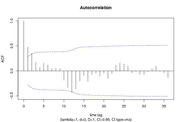
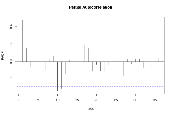
Title produced by software

(Partial) Autocorrelation Function

Date of computation

Tue, 29 Nov 2011 07:10:59 -0500

Cite this page as follows

Statistical Computations at FreeStatistics.org, Office for Research Development and Education, URL https://freestatistics.org/blog/index.php?v=date/2011/Nov/29/t1322568671012ok9nidgqloh6.htm/, Retrieved Thu, 25 Apr 2024 19:51:02 +0000

Statistical Computations at FreeStatistics.org, Office for Research Development and Education, URL https://freestatistics.org/blog/index.php?pk=148228, Retrieved Thu, 25 Apr 2024 19:51:02 +0000

QR Codes:

Paste this QR Code to cite your computation.

Original text written by user:

IsPrivate?

No (this computation is public)

User-defined keywords

Estimated Impact

Family? (F = Feedback message, R = changed R code, M = changed R Module, P = changed Parameters, D = changed Data)

-     [Univariate Explorative Data Analysis] [Run Sequence gebo...] [2008-12-12 13:32:37] [76963dc1903f0f612b6153510a3818cf]
- R  D  [Univariate Explorative Data Analysis] [Run Sequence gebo...] [2008-12-17 12:14:40] [76963dc1903f0f612b6153510a3818cf]
-         [Univariate Explorative Data Analysis] [Run Sequence Plot...] [2008-12-22 18:19:51] [1ce0d16c8f4225c977b42c8fa93bc163]
- RMP       [(Partial) Autocorrelation Function] [Identifying Integ...] [2009-11-22 12:19:56] [b98453cac15ba1066b407e146608df68]
-    D        [(Partial) Autocorrelation Function] [Ws8.2ACF2] [2009-11-25 19:27:24] [e0fc65a5811681d807296d590d5b45de]
-               [(Partial) Autocorrelation Function] [Workshop 8 ACF1] [2010-11-29 17:53:26] [814f53995537cd15c528d8efbf1cf544]
- RM                [(Partial) Autocorrelation Function] [] [2011-11-29 12:10:59] [d41d8cd98f00b204e9800998ecf8427e] [Current]

Feedback Forum

Post a new message

Dataseries X:

Download CSV

Histogram

Boxplots

Summary of computational transaction
Raw Input	view raw input (R code)
Raw Output	view raw output of R engine
Computing time	1 seconds
R Server	'AstonUniversity' @ aston.wessa.net

\begin{tabular}{lllllllll}
\hline
Summary of computational transaction \tabularnewline
Raw Input & view raw input (R code)  \tabularnewline
Raw Output & view raw output of R engine  \tabularnewline
Computing time & 1 seconds \tabularnewline
R Server & 'AstonUniversity' @ aston.wessa.net \tabularnewline
\hline
\end{tabular}
%Source: https://freestatistics.org/blog/index.php?pk=148228&T=0

[TABLE]
[ROW][C]Summary of computational transaction[/C][/ROW]
[ROW][C]Raw Input[/C][C]view raw input (R code) [/C][/ROW]
[ROW][C]Raw Output[/C][C]view raw output of R engine [/C][/ROW]
[ROW][C]Computing time[/C][C]1 seconds[/C][/ROW]
[ROW][C]R Server[/C][C]'AstonUniversity' @ aston.wessa.net[/C][/ROW]
[/TABLE]
Source: https://freestatistics.org/blog/index.php?pk=148228&T=0

Globally Unique Identifier (entire table): ba.freestatistics.org/blog/index.php?pk=148228&T=0

As an alternative you can also use a QR Code:

The GUIDs for individual cells are displayed in the table below:

Summary of computational transaction
Raw Input	view raw input (R code)
Raw Output	view raw output of R engine
Computing time	1 seconds
R Server	'AstonUniversity' @ aston.wessa.net

Autocorrelation Function
Time lag k	ACF(k)	T-STAT	P-value
1	0.479209	3.3201	0.000862
2	0.351099	2.4325	0.009387
3	0.174582	1.2095	0.116189
4	0.072476	0.5021	0.308938
5	0.155777	1.0793	0.142934
6	0.1191	0.8252	0.206684
7	0.049116	0.3403	0.367562
8	0.052504	0.3638	0.358818
9	0.046047	0.319	0.375547
10	-0.185884	-1.2878	0.101988
11	-0.334713	-2.319	0.01235
12	-0.435596	-3.0179	0.002033
13	-0.362122	-2.5089	0.007771
14	-0.203192	-1.4078	0.082824
15	-0.090338	-0.6259	0.267179
16	-0.209836	-1.4538	0.076257
17	-0.069847	-0.4839	0.315323
18	-0.047865	-0.3316	0.37081
19	-0.103752	-0.7188	0.237869
20	-0.045735	-0.3169	0.376362
21	-0.153186	-1.0613	0.146931
22	-0.054213	-0.3756	0.354436
23	0.116261	0.8055	0.212258
24	0.157439	1.0908	0.140409
25	0.139582	0.9671	0.169182
26	0.09635	0.6675	0.253814
27	-0.041642	-0.2885	0.387102
28	-0.010271	-0.0712	0.471783
29	-0.064939	-0.4499	0.327399
30	-0.070301	-0.4871	0.314216
31	-0.014658	-0.1016	0.459768
32	0.040951	0.2837	0.388923
33	0.098599	0.6831	0.248909
34	-0.006323	-0.0438	0.48262
35	-0.041724	-0.2891	0.386885
36	-0.136338	-0.9446	0.174802

\begin{tabular}{lllllllll}
\hline
Autocorrelation Function \tabularnewline
Time lag k & ACF(k) & T-STAT & P-value \tabularnewline
1 & 0.479209 & 3.3201 & 0.000862 \tabularnewline
2 & 0.351099 & 2.4325 & 0.009387 \tabularnewline
3 & 0.174582 & 1.2095 & 0.116189 \tabularnewline
4 & 0.072476 & 0.5021 & 0.308938 \tabularnewline
5 & 0.155777 & 1.0793 & 0.142934 \tabularnewline
6 & 0.1191 & 0.8252 & 0.206684 \tabularnewline
7 & 0.049116 & 0.3403 & 0.367562 \tabularnewline
8 & 0.052504 & 0.3638 & 0.358818 \tabularnewline
9 & 0.046047 & 0.319 & 0.375547 \tabularnewline
10 & -0.185884 & -1.2878 & 0.101988 \tabularnewline
11 & -0.334713 & -2.319 & 0.01235 \tabularnewline
12 & -0.435596 & -3.0179 & 0.002033 \tabularnewline
13 & -0.362122 & -2.5089 & 0.007771 \tabularnewline
14 & -0.203192 & -1.4078 & 0.082824 \tabularnewline
15 & -0.090338 & -0.6259 & 0.267179 \tabularnewline
16 & -0.209836 & -1.4538 & 0.076257 \tabularnewline
17 & -0.069847 & -0.4839 & 0.315323 \tabularnewline
18 & -0.047865 & -0.3316 & 0.37081 \tabularnewline
19 & -0.103752 & -0.7188 & 0.237869 \tabularnewline
20 & -0.045735 & -0.3169 & 0.376362 \tabularnewline
21 & -0.153186 & -1.0613 & 0.146931 \tabularnewline
22 & -0.054213 & -0.3756 & 0.354436 \tabularnewline
23 & 0.116261 & 0.8055 & 0.212258 \tabularnewline
24 & 0.157439 & 1.0908 & 0.140409 \tabularnewline
25 & 0.139582 & 0.9671 & 0.169182 \tabularnewline
26 & 0.09635 & 0.6675 & 0.253814 \tabularnewline
27 & -0.041642 & -0.2885 & 0.387102 \tabularnewline
28 & -0.010271 & -0.0712 & 0.471783 \tabularnewline
29 & -0.064939 & -0.4499 & 0.327399 \tabularnewline
30 & -0.070301 & -0.4871 & 0.314216 \tabularnewline
31 & -0.014658 & -0.1016 & 0.459768 \tabularnewline
32 & 0.040951 & 0.2837 & 0.388923 \tabularnewline
33 & 0.098599 & 0.6831 & 0.248909 \tabularnewline
34 & -0.006323 & -0.0438 & 0.48262 \tabularnewline
35 & -0.041724 & -0.2891 & 0.386885 \tabularnewline
36 & -0.136338 & -0.9446 & 0.174802 \tabularnewline
\hline
\end{tabular}
%Source: https://freestatistics.org/blog/index.php?pk=148228&T=1

[TABLE]
[ROW][C]Autocorrelation Function[/C][/ROW]
[ROW][C]Time lag k[/C][C]ACF(k)[/C][C]T-STAT[/C][C]P-value[/C][/ROW]
[ROW][C]1[/C][C]0.479209[/C][C]3.3201[/C][C]0.000862[/C][/ROW]
[ROW][C]2[/C][C]0.351099[/C][C]2.4325[/C][C]0.009387[/C][/ROW]
[ROW][C]3[/C][C]0.174582[/C][C]1.2095[/C][C]0.116189[/C][/ROW]
[ROW][C]4[/C][C]0.072476[/C][C]0.5021[/C][C]0.308938[/C][/ROW]
[ROW][C]5[/C][C]0.155777[/C][C]1.0793[/C][C]0.142934[/C][/ROW]
[ROW][C]6[/C][C]0.1191[/C][C]0.8252[/C][C]0.206684[/C][/ROW]
[ROW][C]7[/C][C]0.049116[/C][C]0.3403[/C][C]0.367562[/C][/ROW]
[ROW][C]8[/C][C]0.052504[/C][C]0.3638[/C][C]0.358818[/C][/ROW]
[ROW][C]9[/C][C]0.046047[/C][C]0.319[/C][C]0.375547[/C][/ROW]
[ROW][C]10[/C][C]-0.185884[/C][C]-1.2878[/C][C]0.101988[/C][/ROW]
[ROW][C]11[/C][C]-0.334713[/C][C]-2.319[/C][C]0.01235[/C][/ROW]
[ROW][C]12[/C][C]-0.435596[/C][C]-3.0179[/C][C]0.002033[/C][/ROW]
[ROW][C]13[/C][C]-0.362122[/C][C]-2.5089[/C][C]0.007771[/C][/ROW]
[ROW][C]14[/C][C]-0.203192[/C][C]-1.4078[/C][C]0.082824[/C][/ROW]
[ROW][C]15[/C][C]-0.090338[/C][C]-0.6259[/C][C]0.267179[/C][/ROW]
[ROW][C]16[/C][C]-0.209836[/C][C]-1.4538[/C][C]0.076257[/C][/ROW]
[ROW][C]17[/C][C]-0.069847[/C][C]-0.4839[/C][C]0.315323[/C][/ROW]
[ROW][C]18[/C][C]-0.047865[/C][C]-0.3316[/C][C]0.37081[/C][/ROW]
[ROW][C]19[/C][C]-0.103752[/C][C]-0.7188[/C][C]0.237869[/C][/ROW]
[ROW][C]20[/C][C]-0.045735[/C][C]-0.3169[/C][C]0.376362[/C][/ROW]
[ROW][C]21[/C][C]-0.153186[/C][C]-1.0613[/C][C]0.146931[/C][/ROW]
[ROW][C]22[/C][C]-0.054213[/C][C]-0.3756[/C][C]0.354436[/C][/ROW]
[ROW][C]23[/C][C]0.116261[/C][C]0.8055[/C][C]0.212258[/C][/ROW]
[ROW][C]24[/C][C]0.157439[/C][C]1.0908[/C][C]0.140409[/C][/ROW]
[ROW][C]25[/C][C]0.139582[/C][C]0.9671[/C][C]0.169182[/C][/ROW]
[ROW][C]26[/C][C]0.09635[/C][C]0.6675[/C][C]0.253814[/C][/ROW]
[ROW][C]27[/C][C]-0.041642[/C][C]-0.2885[/C][C]0.387102[/C][/ROW]
[ROW][C]28[/C][C]-0.010271[/C][C]-0.0712[/C][C]0.471783[/C][/ROW]
[ROW][C]29[/C][C]-0.064939[/C][C]-0.4499[/C][C]0.327399[/C][/ROW]
[ROW][C]30[/C][C]-0.070301[/C][C]-0.4871[/C][C]0.314216[/C][/ROW]
[ROW][C]31[/C][C]-0.014658[/C][C]-0.1016[/C][C]0.459768[/C][/ROW]
[ROW][C]32[/C][C]0.040951[/C][C]0.2837[/C][C]0.388923[/C][/ROW]
[ROW][C]33[/C][C]0.098599[/C][C]0.6831[/C][C]0.248909[/C][/ROW]
[ROW][C]34[/C][C]-0.006323[/C][C]-0.0438[/C][C]0.48262[/C][/ROW]
[ROW][C]35[/C][C]-0.041724[/C][C]-0.2891[/C][C]0.386885[/C][/ROW]
[ROW][C]36[/C][C]-0.136338[/C][C]-0.9446[/C][C]0.174802[/C][/ROW]
[/TABLE]
Source: https://freestatistics.org/blog/index.php?pk=148228&T=1

Globally Unique Identifier (entire table): ba.freestatistics.org/blog/index.php?pk=148228&T=1

As an alternative you can also use a QR Code:

The GUIDs for individual cells are displayed in the table below:

Autocorrelation Function
Time lag k	ACF(k)	T-STAT	P-value
1	0.479209	3.3201	0.000862
2	0.351099	2.4325	0.009387
3	0.174582	1.2095	0.116189
4	0.072476	0.5021	0.308938
5	0.155777	1.0793	0.142934
6	0.1191	0.8252	0.206684
7	0.049116	0.3403	0.367562
8	0.052504	0.3638	0.358818
9	0.046047	0.319	0.375547
10	-0.185884	-1.2878	0.101988
11	-0.334713	-2.319	0.01235
12	-0.435596	-3.0179	0.002033
13	-0.362122	-2.5089	0.007771
14	-0.203192	-1.4078	0.082824
15	-0.090338	-0.6259	0.267179
16	-0.209836	-1.4538	0.076257
17	-0.069847	-0.4839	0.315323
18	-0.047865	-0.3316	0.37081
19	-0.103752	-0.7188	0.237869
20	-0.045735	-0.3169	0.376362
21	-0.153186	-1.0613	0.146931
22	-0.054213	-0.3756	0.354436
23	0.116261	0.8055	0.212258
24	0.157439	1.0908	0.140409
25	0.139582	0.9671	0.169182
26	0.09635	0.6675	0.253814
27	-0.041642	-0.2885	0.387102
28	-0.010271	-0.0712	0.471783
29	-0.064939	-0.4499	0.327399
30	-0.070301	-0.4871	0.314216
31	-0.014658	-0.1016	0.459768
32	0.040951	0.2837	0.388923
33	0.098599	0.6831	0.248909
34	-0.006323	-0.0438	0.48262
35	-0.041724	-0.2891	0.386885
36	-0.136338	-0.9446	0.174802

Partial Autocorrelation Function
Time lag k	PACF(k)	T-STAT	P-value
1	0.479209	3.3201	0.000862
2	0.157664	1.0923	0.140071
3	-0.056834	-0.3938	0.347752
4	-0.047724	-0.3306	0.371177
5	0.172598	1.1958	0.118826
6	0.014978	0.1038	0.458891
7	-0.097326	-0.6743	0.25168
8	0.032327	0.224	0.411867
9	0.062073	0.4301	0.334541
10	-0.337092	-2.3354	0.011874
11	-0.308932	-2.1403	0.018718
12	-0.144184	-0.9989	0.161418
13	0.022632	0.1568	0.438029
14	0.025179	0.1744	0.431124
15	0.097536	0.6757	0.251222
16	-0.1555	-1.0773	0.143358
17	0.193167	1.3383	0.093551
18	0.154908	1.0732	0.144267
19	-0.111232	-0.7706	0.222349
20	-0.033192	-0.23	0.40955
21	-0.106042	-0.7347	0.233054
22	-0.11362	-0.7872	0.217522
23	-0.036029	-0.2496	0.401975
24	-0.011386	-0.0789	0.468727
25	0.026077	0.1807	0.428694
26	-0.03125	-0.2165	0.414754
27	-0.166274	-1.152	0.127518
28	0.026783	0.1856	0.426785
29	-0.027112	-0.1878	0.425897
30	0.026541	0.1839	0.427441
31	0.026417	0.183	0.427774
32	-0.07084	-0.4908	0.312905
33	0.079062	0.5478	0.293199
34	-0.071858	-0.4978	0.310432
35	-0.037437	-0.2594	0.398229
36	0.036345	0.2518	0.401133

\begin{tabular}{lllllllll}
\hline
Partial Autocorrelation Function \tabularnewline
Time lag k & PACF(k) & T-STAT & P-value \tabularnewline
1 & 0.479209 & 3.3201 & 0.000862 \tabularnewline
2 & 0.157664 & 1.0923 & 0.140071 \tabularnewline
3 & -0.056834 & -0.3938 & 0.347752 \tabularnewline
4 & -0.047724 & -0.3306 & 0.371177 \tabularnewline
5 & 0.172598 & 1.1958 & 0.118826 \tabularnewline
6 & 0.014978 & 0.1038 & 0.458891 \tabularnewline
7 & -0.097326 & -0.6743 & 0.25168 \tabularnewline
8 & 0.032327 & 0.224 & 0.411867 \tabularnewline
9 & 0.062073 & 0.4301 & 0.334541 \tabularnewline
10 & -0.337092 & -2.3354 & 0.011874 \tabularnewline
11 & -0.308932 & -2.1403 & 0.018718 \tabularnewline
12 & -0.144184 & -0.9989 & 0.161418 \tabularnewline
13 & 0.022632 & 0.1568 & 0.438029 \tabularnewline
14 & 0.025179 & 0.1744 & 0.431124 \tabularnewline
15 & 0.097536 & 0.6757 & 0.251222 \tabularnewline
16 & -0.1555 & -1.0773 & 0.143358 \tabularnewline
17 & 0.193167 & 1.3383 & 0.093551 \tabularnewline
18 & 0.154908 & 1.0732 & 0.144267 \tabularnewline
19 & -0.111232 & -0.7706 & 0.222349 \tabularnewline
20 & -0.033192 & -0.23 & 0.40955 \tabularnewline
21 & -0.106042 & -0.7347 & 0.233054 \tabularnewline
22 & -0.11362 & -0.7872 & 0.217522 \tabularnewline
23 & -0.036029 & -0.2496 & 0.401975 \tabularnewline
24 & -0.011386 & -0.0789 & 0.468727 \tabularnewline
25 & 0.026077 & 0.1807 & 0.428694 \tabularnewline
26 & -0.03125 & -0.2165 & 0.414754 \tabularnewline
27 & -0.166274 & -1.152 & 0.127518 \tabularnewline
28 & 0.026783 & 0.1856 & 0.426785 \tabularnewline
29 & -0.027112 & -0.1878 & 0.425897 \tabularnewline
30 & 0.026541 & 0.1839 & 0.427441 \tabularnewline
31 & 0.026417 & 0.183 & 0.427774 \tabularnewline
32 & -0.07084 & -0.4908 & 0.312905 \tabularnewline
33 & 0.079062 & 0.5478 & 0.293199 \tabularnewline
34 & -0.071858 & -0.4978 & 0.310432 \tabularnewline
35 & -0.037437 & -0.2594 & 0.398229 \tabularnewline
36 & 0.036345 & 0.2518 & 0.401133 \tabularnewline
\hline
\end{tabular}
%Source: https://freestatistics.org/blog/index.php?pk=148228&T=2

[TABLE]
[ROW][C]Partial Autocorrelation Function[/C][/ROW]
[ROW][C]Time lag k[/C][C]PACF(k)[/C][C]T-STAT[/C][C]P-value[/C][/ROW]
[ROW][C]1[/C][C]0.479209[/C][C]3.3201[/C][C]0.000862[/C][/ROW]
[ROW][C]2[/C][C]0.157664[/C][C]1.0923[/C][C]0.140071[/C][/ROW]
[ROW][C]3[/C][C]-0.056834[/C][C]-0.3938[/C][C]0.347752[/C][/ROW]
[ROW][C]4[/C][C]-0.047724[/C][C]-0.3306[/C][C]0.371177[/C][/ROW]
[ROW][C]5[/C][C]0.172598[/C][C]1.1958[/C][C]0.118826[/C][/ROW]
[ROW][C]6[/C][C]0.014978[/C][C]0.1038[/C][C]0.458891[/C][/ROW]
[ROW][C]7[/C][C]-0.097326[/C][C]-0.6743[/C][C]0.25168[/C][/ROW]
[ROW][C]8[/C][C]0.032327[/C][C]0.224[/C][C]0.411867[/C][/ROW]
[ROW][C]9[/C][C]0.062073[/C][C]0.4301[/C][C]0.334541[/C][/ROW]
[ROW][C]10[/C][C]-0.337092[/C][C]-2.3354[/C][C]0.011874[/C][/ROW]
[ROW][C]11[/C][C]-0.308932[/C][C]-2.1403[/C][C]0.018718[/C][/ROW]
[ROW][C]12[/C][C]-0.144184[/C][C]-0.9989[/C][C]0.161418[/C][/ROW]
[ROW][C]13[/C][C]0.022632[/C][C]0.1568[/C][C]0.438029[/C][/ROW]
[ROW][C]14[/C][C]0.025179[/C][C]0.1744[/C][C]0.431124[/C][/ROW]
[ROW][C]15[/C][C]0.097536[/C][C]0.6757[/C][C]0.251222[/C][/ROW]
[ROW][C]16[/C][C]-0.1555[/C][C]-1.0773[/C][C]0.143358[/C][/ROW]
[ROW][C]17[/C][C]0.193167[/C][C]1.3383[/C][C]0.093551[/C][/ROW]
[ROW][C]18[/C][C]0.154908[/C][C]1.0732[/C][C]0.144267[/C][/ROW]
[ROW][C]19[/C][C]-0.111232[/C][C]-0.7706[/C][C]0.222349[/C][/ROW]
[ROW][C]20[/C][C]-0.033192[/C][C]-0.23[/C][C]0.40955[/C][/ROW]
[ROW][C]21[/C][C]-0.106042[/C][C]-0.7347[/C][C]0.233054[/C][/ROW]
[ROW][C]22[/C][C]-0.11362[/C][C]-0.7872[/C][C]0.217522[/C][/ROW]
[ROW][C]23[/C][C]-0.036029[/C][C]-0.2496[/C][C]0.401975[/C][/ROW]
[ROW][C]24[/C][C]-0.011386[/C][C]-0.0789[/C][C]0.468727[/C][/ROW]
[ROW][C]25[/C][C]0.026077[/C][C]0.1807[/C][C]0.428694[/C][/ROW]
[ROW][C]26[/C][C]-0.03125[/C][C]-0.2165[/C][C]0.414754[/C][/ROW]
[ROW][C]27[/C][C]-0.166274[/C][C]-1.152[/C][C]0.127518[/C][/ROW]
[ROW][C]28[/C][C]0.026783[/C][C]0.1856[/C][C]0.426785[/C][/ROW]
[ROW][C]29[/C][C]-0.027112[/C][C]-0.1878[/C][C]0.425897[/C][/ROW]
[ROW][C]30[/C][C]0.026541[/C][C]0.1839[/C][C]0.427441[/C][/ROW]
[ROW][C]31[/C][C]0.026417[/C][C]0.183[/C][C]0.427774[/C][/ROW]
[ROW][C]32[/C][C]-0.07084[/C][C]-0.4908[/C][C]0.312905[/C][/ROW]
[ROW][C]33[/C][C]0.079062[/C][C]0.5478[/C][C]0.293199[/C][/ROW]
[ROW][C]34[/C][C]-0.071858[/C][C]-0.4978[/C][C]0.310432[/C][/ROW]
[ROW][C]35[/C][C]-0.037437[/C][C]-0.2594[/C][C]0.398229[/C][/ROW]
[ROW][C]36[/C][C]0.036345[/C][C]0.2518[/C][C]0.401133[/C][/ROW]
[/TABLE]
Source: https://freestatistics.org/blog/index.php?pk=148228&T=2

Globally Unique Identifier (entire table): ba.freestatistics.org/blog/index.php?pk=148228&T=2

As an alternative you can also use a QR Code:

The GUIDs for individual cells are displayed in the table below:

Partial Autocorrelation Function
Time lag k	PACF(k)	T-STAT	P-value
1	0.479209	3.3201	0.000862
2	0.157664	1.0923	0.140071
3	-0.056834	-0.3938	0.347752
4	-0.047724	-0.3306	0.371177
5	0.172598	1.1958	0.118826
6	0.014978	0.1038	0.458891
7	-0.097326	-0.6743	0.25168
8	0.032327	0.224	0.411867
9	0.062073	0.4301	0.334541
10	-0.337092	-2.3354	0.011874
11	-0.308932	-2.1403	0.018718
12	-0.144184	-0.9989	0.161418
13	0.022632	0.1568	0.438029
14	0.025179	0.1744	0.431124
15	0.097536	0.6757	0.251222
16	-0.1555	-1.0773	0.143358
17	0.193167	1.3383	0.093551
18	0.154908	1.0732	0.144267
19	-0.111232	-0.7706	0.222349
20	-0.033192	-0.23	0.40955
21	-0.106042	-0.7347	0.233054
22	-0.11362	-0.7872	0.217522
23	-0.036029	-0.2496	0.401975
24	-0.011386	-0.0789	0.468727
25	0.026077	0.1807	0.428694
26	-0.03125	-0.2165	0.414754
27	-0.166274	-1.152	0.127518
28	0.026783	0.1856	0.426785
29	-0.027112	-0.1878	0.425897
30	0.026541	0.1839	0.427441
31	0.026417	0.183	0.427774
32	-0.07084	-0.4908	0.312905
33	0.079062	0.5478	0.293199
34	-0.071858	-0.4978	0.310432
35	-0.037437	-0.2594	0.398229
36	0.036345	0.2518	0.401133

Figure 1

PNG link

Postscript link

PDF link

Figure 2

PNG link

Postscript link

PDF link

Parameters (Session):

par1 = 36 ; par2 = 1 ; par3 = 0 ; par4 = 1 ; par5 = 12 ; par6 = MA ; par7 = 0.95 ;

Parameters (R input):

par1 = 36 ; par2 = 1 ; par3 = 0 ; par4 = 1 ; par5 = 12 ; par6 = MA ; par7 = 0.95 ; par8 = ; par9 = ; par10 = ; par11 = ; par12 = ; par13 = ; par14 = ; par15 = ; par16 = ; par17 = ; par18 = ; par19 = ; par20 = ;

R code (references can be found in the software module):

if (par1 == 'Default') {
par1 = 10*log10(length(x))
} else {
par1 <- as.numeric(par1)
}
par2 <- as.numeric(par2)
par3 <- as.numeric(par3)
par4 <- as.numeric(par4)
par5 <- as.numeric(par5)
if (par6 == 'White Noise') par6 <- 'white' else par6 <- 'ma'
par7 <- as.numeric(par7)
if (par2 == 0) {
x <- log(x)
} else {
x <- (x ^ par2 - 1) / par2
}
if (par3 > 0) x <- diff(x,lag=1,difference=par3)
if (par4 > 0) x <- diff(x,lag=par5,difference=par4)
bitmap(file='pic1.png')
racf <- acf(x, par1, main='Autocorrelation', xlab='time lag', ylab='ACF', ci.type=par6, ci=par7, sub=paste('(lambda=',par2,', d=',par3,', D=',par4,', CI=', par7, ', CI type=',par6,')',sep=''))
dev.off()
bitmap(file='pic2.png')
rpacf <- pacf(x,par1,main='Partial Autocorrelation',xlab='lags',ylab='PACF')
dev.off()
(myacf <- c(racf$acf))
(mypacf <- c(rpacf$acf))
lengthx <- length(x)
sqrtn <- sqrt(lengthx)
load(file='createtable')
a<-table.start()
a<-table.row.start(a)
a<-table.element(a,'Autocorrelation Function',4,TRUE)
a<-table.row.end(a)
a<-table.row.start(a)
a<-table.element(a,'Time lag k',header=TRUE)
a<-table.element(a,hyperlink('basics.htm','ACF(k)','click here for more information about the Autocorrelation Function'),header=TRUE)
a<-table.element(a,'T-STAT',header=TRUE)
a<-table.element(a,'P-value',header=TRUE)
a<-table.row.end(a)
for (i in 2:(par1+1)) {
a<-table.row.start(a)
a<-table.element(a,i-1,header=TRUE)
a<-table.element(a,round(myacf[i],6))
mytstat <- myacf[i]*sqrtn
a<-table.element(a,round(mytstat,4))
a<-table.element(a,round(1-pt(abs(mytstat),lengthx),6))
a<-table.row.end(a)
}
a<-table.end(a)
table.save(a,file='mytable.tab')
a<-table.start()
a<-table.row.start(a)
a<-table.element(a,'Partial Autocorrelation Function',4,TRUE)
a<-table.row.end(a)
a<-table.row.start(a)
a<-table.element(a,'Time lag k',header=TRUE)
a<-table.element(a,hyperlink('basics.htm','PACF(k)','click here for more information about the Partial Autocorrelation Function'),header=TRUE)
a<-table.element(a,'T-STAT',header=TRUE)
a<-table.element(a,'P-value',header=TRUE)
a<-table.row.end(a)
for (i in 1:par1) {
a<-table.row.start(a)
a<-table.element(a,i,header=TRUE)
a<-table.element(a,round(mypacf[i],6))
mytstat <- mypacf[i]*sqrtn
a<-table.element(a,round(mytstat,4))
a<-table.element(a,round(1-pt(abs(mytstat),lengthx),6))
a<-table.row.end(a)
}
a<-table.end(a)
table.save(a,file='mytable1.tab')

Free Statistics

Description of Statistical Computation

Tree of Dependent Computations

Dataset

Tables (Output of Computation)

Figures (Output of Computation)

Input Parameters & R Code