Free Statistics
of Irreproducible Research!
Description of Statistical Computation | |||||||||||||||||||||
|---|---|---|---|---|---|---|---|---|---|---|---|---|---|---|---|---|---|---|---|---|---|
| Author's title | |||||||||||||||||||||
| Author | *Unverified author* | ||||||||||||||||||||
| R Software Module | rwasp_sdplot.wasp | ||||||||||||||||||||
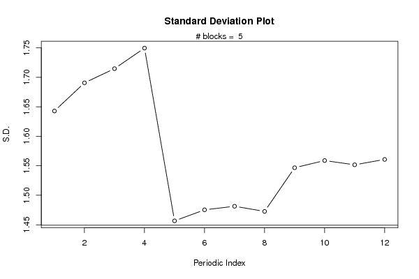
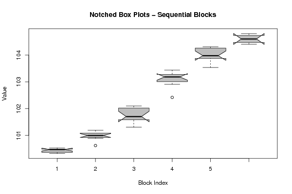
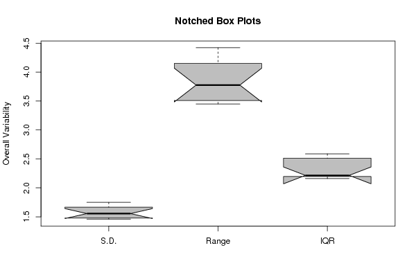
| Title produced by software | Standard Deviation Plot | ||||||||||||||||||||
| Date of computation | Mon, 28 Nov 2011 12:23:21 -0500 | ||||||||||||||||||||
| Cite this page as follows | Statistical Computations at FreeStatistics.org, Office for Research Development and Education, URL https://freestatistics.org/blog/index.php?v=date/2011/Nov/28/t1322501027wf5urdxg4ujrgxw.htm/, Retrieved Fri, 19 Apr 2024 06:12:24 +0000 | ||||||||||||||||||||
| Statistical Computations at FreeStatistics.org, Office for Research Development and Education, URL https://freestatistics.org/blog/index.php?pk=147904, Retrieved Fri, 19 Apr 2024 06:12:24 +0000 | |||||||||||||||||||||
| QR Codes: | |||||||||||||||||||||
|
| |||||||||||||||||||||
| Original text written by user: | |||||||||||||||||||||
| IsPrivate? | No (this computation is public) | ||||||||||||||||||||
| User-defined keywords | KDGP2W83 | ||||||||||||||||||||
| Estimated Impact | 105 | ||||||||||||||||||||
Tree of Dependent Computations | |||||||||||||||||||||
| Family? (F = Feedback message, R = changed R code, M = changed R Module, P = changed Parameters, D = changed Data) | |||||||||||||||||||||
| - [Histogram] [Frequentietabel I...] [2011-11-28 12:49:41] [77b79fca1322508fd7e2d5b3e9715c12] - RMPD [Standard Deviation Plot] [Standard Deviatio...] [2011-11-28 16:08:27] [77b79fca1322508fd7e2d5b3e9715c12] - D [Standard Deviation Plot] [Opdracht3Opgave8] [2011-11-28 17:23:21] [76bda0bb7d6f469fbad64fdea2dd989f] [Current] | |||||||||||||||||||||
| Feedback Forum | |||||||||||||||||||||
Post a new message | |||||||||||||||||||||
Dataset | |||||||||||||||||||||
| Dataseries X: | |||||||||||||||||||||
100,32 100,33 100,35 100,38 100,44 100,47 100,47 100,48 100,48 100,49 100,52 100,53 100,62 100,89 100,92 100,93 100,97 100,98 101,01 101,02 101,07 101,1 101,11 101,19 101,31 101,52 101,56 101,61 101,65 101,66 101,75 101,83 101,98 102,06 102,07 102,1 102,42 102,91 102,91 103,11 103,14 103,14 103,23 103,23 103,26 103,3 103,32 103,44 103,54 103,86 103,88 103,88 103,89 103,98 103,98 103,98 104,24 104,29 104,29 104,31 104,41 104,54 104,67 104,8 | |||||||||||||||||||||
Tables (Output of Computation) | |||||||||||||||||||||
| |||||||||||||||||||||
Figures (Output of Computation) | |||||||||||||||||||||
Input Parameters & R Code | |||||||||||||||||||||
| Parameters (Session): | |||||||||||||||||||||
| par1 = 12 ; | |||||||||||||||||||||
| Parameters (R input): | |||||||||||||||||||||
| par1 = 12 ; | |||||||||||||||||||||
| R code (references can be found in the software module): | |||||||||||||||||||||
par1 <- as.numeric(par1) | |||||||||||||||||||||