Free Statistics
of Irreproducible Research!
Description of Statistical Computation | |||||||||||||||||||||||||||||||||||||||||||||||||||||
|---|---|---|---|---|---|---|---|---|---|---|---|---|---|---|---|---|---|---|---|---|---|---|---|---|---|---|---|---|---|---|---|---|---|---|---|---|---|---|---|---|---|---|---|---|---|---|---|---|---|---|---|---|---|
| Author's title | |||||||||||||||||||||||||||||||||||||||||||||||||||||
| Author | *Unverified author* | ||||||||||||||||||||||||||||||||||||||||||||||||||||
| R Software Module | rwasp_edauni.wasp | ||||||||||||||||||||||||||||||||||||||||||||||||||||
| Title produced by software | Univariate Explorative Data Analysis | ||||||||||||||||||||||||||||||||||||||||||||||||||||
| Date of computation | Thu, 24 Nov 2011 06:53:20 -0500 | ||||||||||||||||||||||||||||||||||||||||||||||||||||
| Cite this page as follows | Statistical Computations at FreeStatistics.org, Office for Research Development and Education, URL https://freestatistics.org/blog/index.php?v=date/2011/Nov/24/t13221356758gcenuyznkhtjb2.htm/, Retrieved Sat, 20 Apr 2024 11:37:36 +0000 | ||||||||||||||||||||||||||||||||||||||||||||||||||||
| Statistical Computations at FreeStatistics.org, Office for Research Development and Education, URL https://freestatistics.org/blog/index.php?pk=146623, Retrieved Sat, 20 Apr 2024 11:37:36 +0000 | |||||||||||||||||||||||||||||||||||||||||||||||||||||
| QR Codes: | |||||||||||||||||||||||||||||||||||||||||||||||||||||
|
| |||||||||||||||||||||||||||||||||||||||||||||||||||||
| Original text written by user: | |||||||||||||||||||||||||||||||||||||||||||||||||||||
| IsPrivate? | No (this computation is public) | ||||||||||||||||||||||||||||||||||||||||||||||||||||
| User-defined keywords | |||||||||||||||||||||||||||||||||||||||||||||||||||||
| Estimated Impact | 136 | ||||||||||||||||||||||||||||||||||||||||||||||||||||
Tree of Dependent Computations | |||||||||||||||||||||||||||||||||||||||||||||||||||||
| Family? (F = Feedback message, R = changed R code, M = changed R Module, P = changed Parameters, D = changed Data) | |||||||||||||||||||||||||||||||||||||||||||||||||||||
| - [Bivariate Data Series] [Bivariate dataset] [2008-01-05 23:51:08] [74be16979710d4c4e7c6647856088456] F RMPD [Univariate Explorative Data Analysis] [Colombia Coffee] [2008-01-07 14:21:11] [74be16979710d4c4e7c6647856088456] - RMPD [Univariate Explorative Data Analysis] [paper] [2011-11-24 11:53:20] [d41d8cd98f00b204e9800998ecf8427e] [Current] - D [Univariate Explorative Data Analysis] [paper] [2011-12-12 11:01:38] [74be16979710d4c4e7c6647856088456] - RMPD [Classical Decomposition] [paper] [2011-12-12 11:46:38] [91ce4971c808115c699d50336245df56] - RMPD [Univariate Data Series] [paper] [2011-12-12 11:48:06] [91ce4971c808115c699d50336245df56] - RMPD [Decomposition by Loess] [paper] [2011-12-12 12:02:29] [91ce4971c808115c699d50336245df56] - RMP [Exponential Smoothing] [Paper] [2011-12-12 12:08:53] [aa6b3f8e5b050429abaad141c7204e84] - RMP [Spectral Analysis] [Paper] [2011-12-12 13:01:06] [aa6b3f8e5b050429abaad141c7204e84] - RMPD [Variance Reduction Matrix] [paper] [2011-12-12 12:45:00] [91ce4971c808115c699d50336245df56] - RMPD [Standard Deviation-Mean Plot] [paper] [2011-12-12 12:50:42] [91ce4971c808115c699d50336245df56] - RMP [ARIMA Backward Selection] [Arima] [2011-12-18 15:33:42] [91ce4971c808115c699d50336245df56] | |||||||||||||||||||||||||||||||||||||||||||||||||||||
| Feedback Forum | |||||||||||||||||||||||||||||||||||||||||||||||||||||
Post a new message | |||||||||||||||||||||||||||||||||||||||||||||||||||||
Dataset | |||||||||||||||||||||||||||||||||||||||||||||||||||||
| Dataseries X: | |||||||||||||||||||||||||||||||||||||||||||||||||||||
68.897 38.683 44.720 39.525 45.315 50.380 40.600 36.279 42.438 38.064 31.879 11.379 70.249 39.253 47.060 41.697 38.708 49.267 39.018 32.228 40.870 39.383 34.571 12.066 70.938 34.077 45.409 40.809 37.013 44.953 37.848 32.745 39.401 34.931 33.008 8.620 68.906 39.556 50.669 36.432 40.891 48.428 36.222 33.425 39.401 37.967 34.801 12.657 69.116 41.519 51.321 38.529 41.547 52.073 38.401 40.898 40.439 41.888 37.898 8.771 68.184 50.530 47.221 41.756 45.633 48.138 39.486 39.341 41.117 41.629 29.722 7.054 56.676 34.870 35.117 30.169 30.936 35.699 33.228 27.733 33.666 35.429 27.438 8.170 63.410 38.040 45.389 37.353 37.024 50.957 37.994 36.454 46.080 43.373 37.395 | |||||||||||||||||||||||||||||||||||||||||||||||||||||
Tables (Output of Computation) | |||||||||||||||||||||||||||||||||||||||||||||||||||||
| |||||||||||||||||||||||||||||||||||||||||||||||||||||
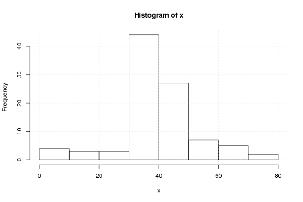
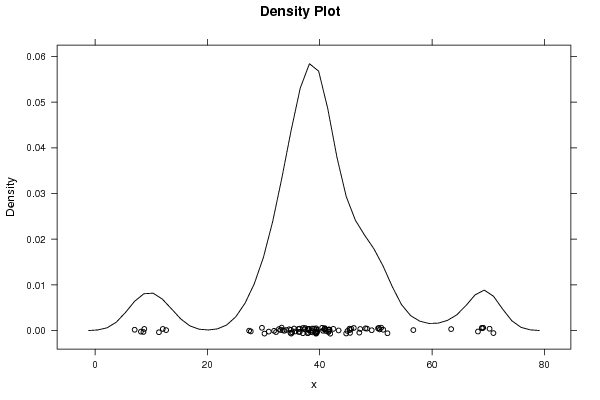
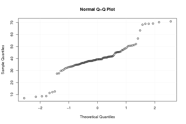
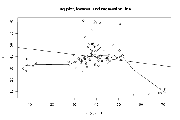
Figures (Output of Computation) | |||||||||||||||||||||||||||||||||||||||||||||||||||||
Input Parameters & R Code | |||||||||||||||||||||||||||||||||||||||||||||||||||||
| Parameters (Session): | |||||||||||||||||||||||||||||||||||||||||||||||||||||
| par1 = 0 ; par2 = 36 ; | |||||||||||||||||||||||||||||||||||||||||||||||||||||
| Parameters (R input): | |||||||||||||||||||||||||||||||||||||||||||||||||||||
| par1 = 0 ; par2 = 36 ; | |||||||||||||||||||||||||||||||||||||||||||||||||||||
| R code (references can be found in the software module): | |||||||||||||||||||||||||||||||||||||||||||||||||||||
par1 <- as.numeric(par1) | |||||||||||||||||||||||||||||||||||||||||||||||||||||