Repository of Reproducible Computations

Free Statistics

of Irreproducible Research!

Author's title

Author

*Unverified author*

R Software Module

rwasp_autocorrelation.wasp

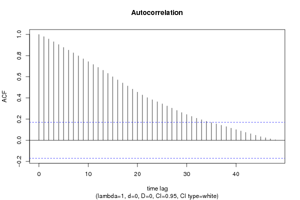
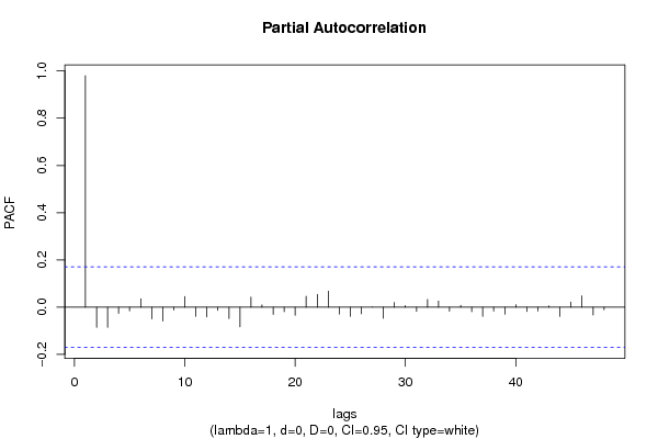
Title produced by software

(Partial) Autocorrelation Function

Date of computation

Wed, 23 Nov 2011 15:56:48 -0500

Cite this page as follows

Statistical Computations at FreeStatistics.org, Office for Research Development and Education, URL https://freestatistics.org/blog/index.php?v=date/2011/Nov/23/t1322081893szr7w4wpfr07wej.htm/, Retrieved Fri, 26 Apr 2024 22:29:04 +0000

Statistical Computations at FreeStatistics.org, Office for Research Development and Education, URL https://freestatistics.org/blog/index.php?pk=146587, Retrieved Fri, 26 Apr 2024 22:29:04 +0000

QR Codes:

Paste this QR Code to cite your computation.

Original text written by user:

IsPrivate?

No (this computation is public)

User-defined keywords

KDGP2W12

Estimated Impact

Family? (F = Feedback message, R = changed R code, M = changed R Module, P = changed Parameters, D = changed Data)

-       [(Partial) Autocorrelation Function] [] [2011-11-23 20:56:48] [860f1af8dde2fbc4c0f468abef92388b] [Current]

Feedback Forum

Post a new message

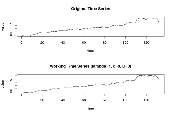
Dataseries X:

Download CSV

Histogram

Boxplots

Summary of computational transaction
Raw Input	view raw input (R code)
Raw Output	view raw output of R engine
Computing time	2 seconds
R Server	'AstonUniversity' @ aston.wessa.net

\begin{tabular}{lllllllll}
\hline
Summary of computational transaction \tabularnewline
Raw Input & view raw input (R code)  \tabularnewline
Raw Output & view raw output of R engine  \tabularnewline
Computing time & 2 seconds \tabularnewline
R Server & 'AstonUniversity' @ aston.wessa.net \tabularnewline
\hline
\end{tabular}
%Source: https://freestatistics.org/blog/index.php?pk=146587&T=0

[TABLE]
[ROW][C]Summary of computational transaction[/C][/ROW]
[ROW][C]Raw Input[/C][C]view raw input (R code) [/C][/ROW]
[ROW][C]Raw Output[/C][C]view raw output of R engine [/C][/ROW]
[ROW][C]Computing time[/C][C]2 seconds[/C][/ROW]
[ROW][C]R Server[/C][C]'AstonUniversity' @ aston.wessa.net[/C][/ROW]
[/TABLE]
Source: https://freestatistics.org/blog/index.php?pk=146587&T=0

Globally Unique Identifier (entire table): ba.freestatistics.org/blog/index.php?pk=146587&T=0

As an alternative you can also use a QR Code:

The GUIDs for individual cells are displayed in the table below:

Summary of computational transaction
Raw Input	view raw input (R code)
Raw Output	view raw output of R engine
Computing time	2 seconds
R Server	'AstonUniversity' @ aston.wessa.net

Autocorrelation Function
Time lag k	ACF(k)	T-STAT	P-value
1	0.980201	11.2617	0
2	0.957459	11.0004	0
3	0.931625	10.7036	0
4	0.90488	10.3963	0
5	0.877755	10.0846	0
6	0.85245	9.7939	0
7	0.825964	9.4896	0
8	0.797902	9.1672	0
9	0.769641	8.8425	0
10	0.743464	8.5418	0
11	0.716475	8.2317	0
12	0.688844	7.9142	0
13	0.661304	7.5978	0
14	0.632337	7.265	0
15	0.600381	6.8978	0
16	0.570466	6.5542	0
17	0.541679	6.2234	0
18	0.512695	5.8904	0
19	0.483884	5.5594	0
20	0.454829	5.2256	0
21	0.427806	4.9151	1e-06
22	0.40347	4.6355	4e-06
23	0.383422	4.4052	1.1e-05
24	0.364191	4.1842	2.6e-05
25	0.344431	3.9572	6.2e-05
26	0.323933	3.7217	0.000146
27	0.303804	3.4904	0.000328
28	0.282166	3.2418	0.000752
29	0.262201	3.0125	0.001553
30	0.243682	2.7997	0.002942
31	0.225368	2.5893	0.005348
32	0.208611	2.3968	0.008971
33	0.193888	2.2276	0.0138
34	0.179582	2.0632	0.020525
35	0.166862	1.9171	0.028693
36	0.154716	1.7775	0.03889
37	0.14218	1.6335	0.052371
38	0.128771	1.4795	0.0707
39	0.114406	1.3144	0.095491
40	0.101119	1.1618	0.123713
41	0.087722	1.0078	0.157687
42	0.074171	0.8522	0.197834
43	0.061428	0.7058	0.240793
44	0.047371	0.5443	0.293593
45	0.034069	0.3914	0.348059
46	0.023626	0.2714	0.393237
47	0.013291	0.1527	0.439433
48	0.003586	0.0412	0.483601

\begin{tabular}{lllllllll}
\hline
Autocorrelation Function \tabularnewline
Time lag k & ACF(k) & T-STAT & P-value \tabularnewline
1 & 0.980201 & 11.2617 & 0 \tabularnewline
2 & 0.957459 & 11.0004 & 0 \tabularnewline
3 & 0.931625 & 10.7036 & 0 \tabularnewline
4 & 0.90488 & 10.3963 & 0 \tabularnewline
5 & 0.877755 & 10.0846 & 0 \tabularnewline
6 & 0.85245 & 9.7939 & 0 \tabularnewline
7 & 0.825964 & 9.4896 & 0 \tabularnewline
8 & 0.797902 & 9.1672 & 0 \tabularnewline
9 & 0.769641 & 8.8425 & 0 \tabularnewline
10 & 0.743464 & 8.5418 & 0 \tabularnewline
11 & 0.716475 & 8.2317 & 0 \tabularnewline
12 & 0.688844 & 7.9142 & 0 \tabularnewline
13 & 0.661304 & 7.5978 & 0 \tabularnewline
14 & 0.632337 & 7.265 & 0 \tabularnewline
15 & 0.600381 & 6.8978 & 0 \tabularnewline
16 & 0.570466 & 6.5542 & 0 \tabularnewline
17 & 0.541679 & 6.2234 & 0 \tabularnewline
18 & 0.512695 & 5.8904 & 0 \tabularnewline
19 & 0.483884 & 5.5594 & 0 \tabularnewline
20 & 0.454829 & 5.2256 & 0 \tabularnewline
21 & 0.427806 & 4.9151 & 1e-06 \tabularnewline
22 & 0.40347 & 4.6355 & 4e-06 \tabularnewline
23 & 0.383422 & 4.4052 & 1.1e-05 \tabularnewline
24 & 0.364191 & 4.1842 & 2.6e-05 \tabularnewline
25 & 0.344431 & 3.9572 & 6.2e-05 \tabularnewline
26 & 0.323933 & 3.7217 & 0.000146 \tabularnewline
27 & 0.303804 & 3.4904 & 0.000328 \tabularnewline
28 & 0.282166 & 3.2418 & 0.000752 \tabularnewline
29 & 0.262201 & 3.0125 & 0.001553 \tabularnewline
30 & 0.243682 & 2.7997 & 0.002942 \tabularnewline
31 & 0.225368 & 2.5893 & 0.005348 \tabularnewline
32 & 0.208611 & 2.3968 & 0.008971 \tabularnewline
33 & 0.193888 & 2.2276 & 0.0138 \tabularnewline
34 & 0.179582 & 2.0632 & 0.020525 \tabularnewline
35 & 0.166862 & 1.9171 & 0.028693 \tabularnewline
36 & 0.154716 & 1.7775 & 0.03889 \tabularnewline
37 & 0.14218 & 1.6335 & 0.052371 \tabularnewline
38 & 0.128771 & 1.4795 & 0.0707 \tabularnewline
39 & 0.114406 & 1.3144 & 0.095491 \tabularnewline
40 & 0.101119 & 1.1618 & 0.123713 \tabularnewline
41 & 0.087722 & 1.0078 & 0.157687 \tabularnewline
42 & 0.074171 & 0.8522 & 0.197834 \tabularnewline
43 & 0.061428 & 0.7058 & 0.240793 \tabularnewline
44 & 0.047371 & 0.5443 & 0.293593 \tabularnewline
45 & 0.034069 & 0.3914 & 0.348059 \tabularnewline
46 & 0.023626 & 0.2714 & 0.393237 \tabularnewline
47 & 0.013291 & 0.1527 & 0.439433 \tabularnewline
48 & 0.003586 & 0.0412 & 0.483601 \tabularnewline
\hline
\end{tabular}
%Source: https://freestatistics.org/blog/index.php?pk=146587&T=1

[TABLE]
[ROW][C]Autocorrelation Function[/C][/ROW]
[ROW][C]Time lag k[/C][C]ACF(k)[/C][C]T-STAT[/C][C]P-value[/C][/ROW]
[ROW][C]1[/C][C]0.980201[/C][C]11.2617[/C][C]0[/C][/ROW]
[ROW][C]2[/C][C]0.957459[/C][C]11.0004[/C][C]0[/C][/ROW]
[ROW][C]3[/C][C]0.931625[/C][C]10.7036[/C][C]0[/C][/ROW]
[ROW][C]4[/C][C]0.90488[/C][C]10.3963[/C][C]0[/C][/ROW]
[ROW][C]5[/C][C]0.877755[/C][C]10.0846[/C][C]0[/C][/ROW]
[ROW][C]6[/C][C]0.85245[/C][C]9.7939[/C][C]0[/C][/ROW]
[ROW][C]7[/C][C]0.825964[/C][C]9.4896[/C][C]0[/C][/ROW]
[ROW][C]8[/C][C]0.797902[/C][C]9.1672[/C][C]0[/C][/ROW]
[ROW][C]9[/C][C]0.769641[/C][C]8.8425[/C][C]0[/C][/ROW]
[ROW][C]10[/C][C]0.743464[/C][C]8.5418[/C][C]0[/C][/ROW]
[ROW][C]11[/C][C]0.716475[/C][C]8.2317[/C][C]0[/C][/ROW]
[ROW][C]12[/C][C]0.688844[/C][C]7.9142[/C][C]0[/C][/ROW]
[ROW][C]13[/C][C]0.661304[/C][C]7.5978[/C][C]0[/C][/ROW]
[ROW][C]14[/C][C]0.632337[/C][C]7.265[/C][C]0[/C][/ROW]
[ROW][C]15[/C][C]0.600381[/C][C]6.8978[/C][C]0[/C][/ROW]
[ROW][C]16[/C][C]0.570466[/C][C]6.5542[/C][C]0[/C][/ROW]
[ROW][C]17[/C][C]0.541679[/C][C]6.2234[/C][C]0[/C][/ROW]
[ROW][C]18[/C][C]0.512695[/C][C]5.8904[/C][C]0[/C][/ROW]
[ROW][C]19[/C][C]0.483884[/C][C]5.5594[/C][C]0[/C][/ROW]
[ROW][C]20[/C][C]0.454829[/C][C]5.2256[/C][C]0[/C][/ROW]
[ROW][C]21[/C][C]0.427806[/C][C]4.9151[/C][C]1e-06[/C][/ROW]
[ROW][C]22[/C][C]0.40347[/C][C]4.6355[/C][C]4e-06[/C][/ROW]
[ROW][C]23[/C][C]0.383422[/C][C]4.4052[/C][C]1.1e-05[/C][/ROW]
[ROW][C]24[/C][C]0.364191[/C][C]4.1842[/C][C]2.6e-05[/C][/ROW]
[ROW][C]25[/C][C]0.344431[/C][C]3.9572[/C][C]6.2e-05[/C][/ROW]
[ROW][C]26[/C][C]0.323933[/C][C]3.7217[/C][C]0.000146[/C][/ROW]
[ROW][C]27[/C][C]0.303804[/C][C]3.4904[/C][C]0.000328[/C][/ROW]
[ROW][C]28[/C][C]0.282166[/C][C]3.2418[/C][C]0.000752[/C][/ROW]
[ROW][C]29[/C][C]0.262201[/C][C]3.0125[/C][C]0.001553[/C][/ROW]
[ROW][C]30[/C][C]0.243682[/C][C]2.7997[/C][C]0.002942[/C][/ROW]
[ROW][C]31[/C][C]0.225368[/C][C]2.5893[/C][C]0.005348[/C][/ROW]
[ROW][C]32[/C][C]0.208611[/C][C]2.3968[/C][C]0.008971[/C][/ROW]
[ROW][C]33[/C][C]0.193888[/C][C]2.2276[/C][C]0.0138[/C][/ROW]
[ROW][C]34[/C][C]0.179582[/C][C]2.0632[/C][C]0.020525[/C][/ROW]
[ROW][C]35[/C][C]0.166862[/C][C]1.9171[/C][C]0.028693[/C][/ROW]
[ROW][C]36[/C][C]0.154716[/C][C]1.7775[/C][C]0.03889[/C][/ROW]
[ROW][C]37[/C][C]0.14218[/C][C]1.6335[/C][C]0.052371[/C][/ROW]
[ROW][C]38[/C][C]0.128771[/C][C]1.4795[/C][C]0.0707[/C][/ROW]
[ROW][C]39[/C][C]0.114406[/C][C]1.3144[/C][C]0.095491[/C][/ROW]
[ROW][C]40[/C][C]0.101119[/C][C]1.1618[/C][C]0.123713[/C][/ROW]
[ROW][C]41[/C][C]0.087722[/C][C]1.0078[/C][C]0.157687[/C][/ROW]
[ROW][C]42[/C][C]0.074171[/C][C]0.8522[/C][C]0.197834[/C][/ROW]
[ROW][C]43[/C][C]0.061428[/C][C]0.7058[/C][C]0.240793[/C][/ROW]
[ROW][C]44[/C][C]0.047371[/C][C]0.5443[/C][C]0.293593[/C][/ROW]
[ROW][C]45[/C][C]0.034069[/C][C]0.3914[/C][C]0.348059[/C][/ROW]
[ROW][C]46[/C][C]0.023626[/C][C]0.2714[/C][C]0.393237[/C][/ROW]
[ROW][C]47[/C][C]0.013291[/C][C]0.1527[/C][C]0.439433[/C][/ROW]
[ROW][C]48[/C][C]0.003586[/C][C]0.0412[/C][C]0.483601[/C][/ROW]
[/TABLE]
Source: https://freestatistics.org/blog/index.php?pk=146587&T=1

Globally Unique Identifier (entire table): ba.freestatistics.org/blog/index.php?pk=146587&T=1

As an alternative you can also use a QR Code:

The GUIDs for individual cells are displayed in the table below:

Autocorrelation Function
Time lag k	ACF(k)	T-STAT	P-value
1	0.980201	11.2617	0
2	0.957459	11.0004	0
3	0.931625	10.7036	0
4	0.90488	10.3963	0
5	0.877755	10.0846	0
6	0.85245	9.7939	0
7	0.825964	9.4896	0
8	0.797902	9.1672	0
9	0.769641	8.8425	0
10	0.743464	8.5418	0
11	0.716475	8.2317	0
12	0.688844	7.9142	0
13	0.661304	7.5978	0
14	0.632337	7.265	0
15	0.600381	6.8978	0
16	0.570466	6.5542	0
17	0.541679	6.2234	0
18	0.512695	5.8904	0
19	0.483884	5.5594	0
20	0.454829	5.2256	0
21	0.427806	4.9151	1e-06
22	0.40347	4.6355	4e-06
23	0.383422	4.4052	1.1e-05
24	0.364191	4.1842	2.6e-05
25	0.344431	3.9572	6.2e-05
26	0.323933	3.7217	0.000146
27	0.303804	3.4904	0.000328
28	0.282166	3.2418	0.000752
29	0.262201	3.0125	0.001553
30	0.243682	2.7997	0.002942
31	0.225368	2.5893	0.005348
32	0.208611	2.3968	0.008971
33	0.193888	2.2276	0.0138
34	0.179582	2.0632	0.020525
35	0.166862	1.9171	0.028693
36	0.154716	1.7775	0.03889
37	0.14218	1.6335	0.052371
38	0.128771	1.4795	0.0707
39	0.114406	1.3144	0.095491
40	0.101119	1.1618	0.123713
41	0.087722	1.0078	0.157687
42	0.074171	0.8522	0.197834
43	0.061428	0.7058	0.240793
44	0.047371	0.5443	0.293593
45	0.034069	0.3914	0.348059
46	0.023626	0.2714	0.393237
47	0.013291	0.1527	0.439433
48	0.003586	0.0412	0.483601

Partial Autocorrelation Function
Time lag k	PACF(k)	T-STAT	P-value
1	0.980201	11.2617	0
2	-0.085099	-0.9777	0.165004
3	-0.085523	-0.9826	0.163806
4	-0.026292	-0.3021	0.381537
5	-0.015854	-0.1822	0.427871
6	0.036047	0.4142	0.339717
7	-0.049554	-0.5693	0.285048
8	-0.058094	-0.6674	0.252825
9	-0.012278	-0.1411	0.444018
10	0.045362	0.5212	0.301562
11	-0.039083	-0.449	0.327073
12	-0.041178	-0.4731	0.318461
13	-0.013513	-0.1553	0.43843
14	-0.048146	-0.5532	0.290545
15	-0.083325	-0.9573	0.170075
16	0.042433	0.4875	0.313351
17	0.009822	0.1129	0.45516
18	-0.031058	-0.3568	0.360895
19	-0.018635	-0.2141	0.415402
20	-0.034164	-0.3925	0.347658
21	0.046151	0.5302	0.29842
22	0.053812	0.6183	0.268735
23	0.067817	0.7792	0.218641
24	-0.028836	-0.3313	0.370472
25	-0.03887	-0.4466	0.327954
26	-0.027884	-0.3204	0.374601
27	-0.000202	-0.0023	0.499074
28	-0.047191	-0.5422	0.294305
29	0.020287	0.2331	0.408032
30	0.007003	0.0805	0.467997
31	-0.017191	-0.1975	0.421866
32	0.033027	0.3794	0.352482
33	0.026042	0.2992	0.382627
34	-0.016981	-0.1951	0.422808
35	0.007675	0.0882	0.464935
36	-0.018766	-0.2156	0.414815
37	-0.038428	-0.4415	0.329787
38	-0.016173	-0.1858	0.42644
39	-0.029295	-0.3366	0.368486
40	0.010979	0.1261	0.449905
41	-0.018032	-0.2072	0.418096
42	-0.016063	-0.1846	0.426932
43	0.00591	0.0679	0.472986
44	-0.038385	-0.441	0.329964
45	0.022321	0.2564	0.399002
46	0.04799	0.5514	0.291159
47	-0.033387	-0.3836	0.350952
48	-0.010484	-0.1205	0.452155

\begin{tabular}{lllllllll}
\hline
Partial Autocorrelation Function \tabularnewline
Time lag k & PACF(k) & T-STAT & P-value \tabularnewline
1 & 0.980201 & 11.2617 & 0 \tabularnewline
2 & -0.085099 & -0.9777 & 0.165004 \tabularnewline
3 & -0.085523 & -0.9826 & 0.163806 \tabularnewline
4 & -0.026292 & -0.3021 & 0.381537 \tabularnewline
5 & -0.015854 & -0.1822 & 0.427871 \tabularnewline
6 & 0.036047 & 0.4142 & 0.339717 \tabularnewline
7 & -0.049554 & -0.5693 & 0.285048 \tabularnewline
8 & -0.058094 & -0.6674 & 0.252825 \tabularnewline
9 & -0.012278 & -0.1411 & 0.444018 \tabularnewline
10 & 0.045362 & 0.5212 & 0.301562 \tabularnewline
11 & -0.039083 & -0.449 & 0.327073 \tabularnewline
12 & -0.041178 & -0.4731 & 0.318461 \tabularnewline
13 & -0.013513 & -0.1553 & 0.43843 \tabularnewline
14 & -0.048146 & -0.5532 & 0.290545 \tabularnewline
15 & -0.083325 & -0.9573 & 0.170075 \tabularnewline
16 & 0.042433 & 0.4875 & 0.313351 \tabularnewline
17 & 0.009822 & 0.1129 & 0.45516 \tabularnewline
18 & -0.031058 & -0.3568 & 0.360895 \tabularnewline
19 & -0.018635 & -0.2141 & 0.415402 \tabularnewline
20 & -0.034164 & -0.3925 & 0.347658 \tabularnewline
21 & 0.046151 & 0.5302 & 0.29842 \tabularnewline
22 & 0.053812 & 0.6183 & 0.268735 \tabularnewline
23 & 0.067817 & 0.7792 & 0.218641 \tabularnewline
24 & -0.028836 & -0.3313 & 0.370472 \tabularnewline
25 & -0.03887 & -0.4466 & 0.327954 \tabularnewline
26 & -0.027884 & -0.3204 & 0.374601 \tabularnewline
27 & -0.000202 & -0.0023 & 0.499074 \tabularnewline
28 & -0.047191 & -0.5422 & 0.294305 \tabularnewline
29 & 0.020287 & 0.2331 & 0.408032 \tabularnewline
30 & 0.007003 & 0.0805 & 0.467997 \tabularnewline
31 & -0.017191 & -0.1975 & 0.421866 \tabularnewline
32 & 0.033027 & 0.3794 & 0.352482 \tabularnewline
33 & 0.026042 & 0.2992 & 0.382627 \tabularnewline
34 & -0.016981 & -0.1951 & 0.422808 \tabularnewline
35 & 0.007675 & 0.0882 & 0.464935 \tabularnewline
36 & -0.018766 & -0.2156 & 0.414815 \tabularnewline
37 & -0.038428 & -0.4415 & 0.329787 \tabularnewline
38 & -0.016173 & -0.1858 & 0.42644 \tabularnewline
39 & -0.029295 & -0.3366 & 0.368486 \tabularnewline
40 & 0.010979 & 0.1261 & 0.449905 \tabularnewline
41 & -0.018032 & -0.2072 & 0.418096 \tabularnewline
42 & -0.016063 & -0.1846 & 0.426932 \tabularnewline
43 & 0.00591 & 0.0679 & 0.472986 \tabularnewline
44 & -0.038385 & -0.441 & 0.329964 \tabularnewline
45 & 0.022321 & 0.2564 & 0.399002 \tabularnewline
46 & 0.04799 & 0.5514 & 0.291159 \tabularnewline
47 & -0.033387 & -0.3836 & 0.350952 \tabularnewline
48 & -0.010484 & -0.1205 & 0.452155 \tabularnewline
\hline
\end{tabular}
%Source: https://freestatistics.org/blog/index.php?pk=146587&T=2

[TABLE]
[ROW][C]Partial Autocorrelation Function[/C][/ROW]
[ROW][C]Time lag k[/C][C]PACF(k)[/C][C]T-STAT[/C][C]P-value[/C][/ROW]
[ROW][C]1[/C][C]0.980201[/C][C]11.2617[/C][C]0[/C][/ROW]
[ROW][C]2[/C][C]-0.085099[/C][C]-0.9777[/C][C]0.165004[/C][/ROW]
[ROW][C]3[/C][C]-0.085523[/C][C]-0.9826[/C][C]0.163806[/C][/ROW]
[ROW][C]4[/C][C]-0.026292[/C][C]-0.3021[/C][C]0.381537[/C][/ROW]
[ROW][C]5[/C][C]-0.015854[/C][C]-0.1822[/C][C]0.427871[/C][/ROW]
[ROW][C]6[/C][C]0.036047[/C][C]0.4142[/C][C]0.339717[/C][/ROW]
[ROW][C]7[/C][C]-0.049554[/C][C]-0.5693[/C][C]0.285048[/C][/ROW]
[ROW][C]8[/C][C]-0.058094[/C][C]-0.6674[/C][C]0.252825[/C][/ROW]
[ROW][C]9[/C][C]-0.012278[/C][C]-0.1411[/C][C]0.444018[/C][/ROW]
[ROW][C]10[/C][C]0.045362[/C][C]0.5212[/C][C]0.301562[/C][/ROW]
[ROW][C]11[/C][C]-0.039083[/C][C]-0.449[/C][C]0.327073[/C][/ROW]
[ROW][C]12[/C][C]-0.041178[/C][C]-0.4731[/C][C]0.318461[/C][/ROW]
[ROW][C]13[/C][C]-0.013513[/C][C]-0.1553[/C][C]0.43843[/C][/ROW]
[ROW][C]14[/C][C]-0.048146[/C][C]-0.5532[/C][C]0.290545[/C][/ROW]
[ROW][C]15[/C][C]-0.083325[/C][C]-0.9573[/C][C]0.170075[/C][/ROW]
[ROW][C]16[/C][C]0.042433[/C][C]0.4875[/C][C]0.313351[/C][/ROW]
[ROW][C]17[/C][C]0.009822[/C][C]0.1129[/C][C]0.45516[/C][/ROW]
[ROW][C]18[/C][C]-0.031058[/C][C]-0.3568[/C][C]0.360895[/C][/ROW]
[ROW][C]19[/C][C]-0.018635[/C][C]-0.2141[/C][C]0.415402[/C][/ROW]
[ROW][C]20[/C][C]-0.034164[/C][C]-0.3925[/C][C]0.347658[/C][/ROW]
[ROW][C]21[/C][C]0.046151[/C][C]0.5302[/C][C]0.29842[/C][/ROW]
[ROW][C]22[/C][C]0.053812[/C][C]0.6183[/C][C]0.268735[/C][/ROW]
[ROW][C]23[/C][C]0.067817[/C][C]0.7792[/C][C]0.218641[/C][/ROW]
[ROW][C]24[/C][C]-0.028836[/C][C]-0.3313[/C][C]0.370472[/C][/ROW]
[ROW][C]25[/C][C]-0.03887[/C][C]-0.4466[/C][C]0.327954[/C][/ROW]
[ROW][C]26[/C][C]-0.027884[/C][C]-0.3204[/C][C]0.374601[/C][/ROW]
[ROW][C]27[/C][C]-0.000202[/C][C]-0.0023[/C][C]0.499074[/C][/ROW]
[ROW][C]28[/C][C]-0.047191[/C][C]-0.5422[/C][C]0.294305[/C][/ROW]
[ROW][C]29[/C][C]0.020287[/C][C]0.2331[/C][C]0.408032[/C][/ROW]
[ROW][C]30[/C][C]0.007003[/C][C]0.0805[/C][C]0.467997[/C][/ROW]
[ROW][C]31[/C][C]-0.017191[/C][C]-0.1975[/C][C]0.421866[/C][/ROW]
[ROW][C]32[/C][C]0.033027[/C][C]0.3794[/C][C]0.352482[/C][/ROW]
[ROW][C]33[/C][C]0.026042[/C][C]0.2992[/C][C]0.382627[/C][/ROW]
[ROW][C]34[/C][C]-0.016981[/C][C]-0.1951[/C][C]0.422808[/C][/ROW]
[ROW][C]35[/C][C]0.007675[/C][C]0.0882[/C][C]0.464935[/C][/ROW]
[ROW][C]36[/C][C]-0.018766[/C][C]-0.2156[/C][C]0.414815[/C][/ROW]
[ROW][C]37[/C][C]-0.038428[/C][C]-0.4415[/C][C]0.329787[/C][/ROW]
[ROW][C]38[/C][C]-0.016173[/C][C]-0.1858[/C][C]0.42644[/C][/ROW]
[ROW][C]39[/C][C]-0.029295[/C][C]-0.3366[/C][C]0.368486[/C][/ROW]
[ROW][C]40[/C][C]0.010979[/C][C]0.1261[/C][C]0.449905[/C][/ROW]
[ROW][C]41[/C][C]-0.018032[/C][C]-0.2072[/C][C]0.418096[/C][/ROW]
[ROW][C]42[/C][C]-0.016063[/C][C]-0.1846[/C][C]0.426932[/C][/ROW]
[ROW][C]43[/C][C]0.00591[/C][C]0.0679[/C][C]0.472986[/C][/ROW]
[ROW][C]44[/C][C]-0.038385[/C][C]-0.441[/C][C]0.329964[/C][/ROW]
[ROW][C]45[/C][C]0.022321[/C][C]0.2564[/C][C]0.399002[/C][/ROW]
[ROW][C]46[/C][C]0.04799[/C][C]0.5514[/C][C]0.291159[/C][/ROW]
[ROW][C]47[/C][C]-0.033387[/C][C]-0.3836[/C][C]0.350952[/C][/ROW]
[ROW][C]48[/C][C]-0.010484[/C][C]-0.1205[/C][C]0.452155[/C][/ROW]
[/TABLE]
Source: https://freestatistics.org/blog/index.php?pk=146587&T=2

Globally Unique Identifier (entire table): ba.freestatistics.org/blog/index.php?pk=146587&T=2

As an alternative you can also use a QR Code:

The GUIDs for individual cells are displayed in the table below:

Partial Autocorrelation Function
Time lag k	PACF(k)	T-STAT	P-value
1	0.980201	11.2617	0
2	-0.085099	-0.9777	0.165004
3	-0.085523	-0.9826	0.163806
4	-0.026292	-0.3021	0.381537
5	-0.015854	-0.1822	0.427871
6	0.036047	0.4142	0.339717
7	-0.049554	-0.5693	0.285048
8	-0.058094	-0.6674	0.252825
9	-0.012278	-0.1411	0.444018
10	0.045362	0.5212	0.301562
11	-0.039083	-0.449	0.327073
12	-0.041178	-0.4731	0.318461
13	-0.013513	-0.1553	0.43843
14	-0.048146	-0.5532	0.290545
15	-0.083325	-0.9573	0.170075
16	0.042433	0.4875	0.313351
17	0.009822	0.1129	0.45516
18	-0.031058	-0.3568	0.360895
19	-0.018635	-0.2141	0.415402
20	-0.034164	-0.3925	0.347658
21	0.046151	0.5302	0.29842
22	0.053812	0.6183	0.268735
23	0.067817	0.7792	0.218641
24	-0.028836	-0.3313	0.370472
25	-0.03887	-0.4466	0.327954
26	-0.027884	-0.3204	0.374601
27	-0.000202	-0.0023	0.499074
28	-0.047191	-0.5422	0.294305
29	0.020287	0.2331	0.408032
30	0.007003	0.0805	0.467997
31	-0.017191	-0.1975	0.421866
32	0.033027	0.3794	0.352482
33	0.026042	0.2992	0.382627
34	-0.016981	-0.1951	0.422808
35	0.007675	0.0882	0.464935
36	-0.018766	-0.2156	0.414815
37	-0.038428	-0.4415	0.329787
38	-0.016173	-0.1858	0.42644
39	-0.029295	-0.3366	0.368486
40	0.010979	0.1261	0.449905
41	-0.018032	-0.2072	0.418096
42	-0.016063	-0.1846	0.426932
43	0.00591	0.0679	0.472986
44	-0.038385	-0.441	0.329964
45	0.022321	0.2564	0.399002
46	0.04799	0.5514	0.291159
47	-0.033387	-0.3836	0.350952
48	-0.010484	-0.1205	0.452155

Figure 1

PNG link

Postscript link

PDF link

Figure 2

PNG link

Postscript link

PDF link

Figure 3

PNG link

Postscript link

PDF link

Parameters (Session):

par1 = 48 ; par2 = 1 ; par3 = 0 ; par4 = 0 ; par5 = 12 ; par6 = White Noise ; par7 = 0.95 ;

Parameters (R input):

par1 = 48 ; par2 = 1 ; par3 = 0 ; par4 = 0 ; par5 = 12 ; par6 = White Noise ; par7 = 0.95 ; par8 = ;

R code (references can be found in the software module):

if (par1 == 'Default') {
par1 = 10*log10(length(x))
} else {
par1 <- as.numeric(par1)
}
par2 <- as.numeric(par2)
par3 <- as.numeric(par3)
par4 <- as.numeric(par4)
par5 <- as.numeric(par5)
if (par6 == 'White Noise') par6 <- 'white' else par6 <- 'ma'
par7 <- as.numeric(par7)
if (par8 != '') par8 <- as.numeric(par8)
ox <- x
if (par8 == '') {
if (par2 == 0) {
x <- log(x)
} else {
x <- (x ^ par2 - 1) / par2
}
} else {
x <- log(x,base=par8)
}
if (par3 > 0) x <- diff(x,lag=1,difference=par3)
if (par4 > 0) x <- diff(x,lag=par5,difference=par4)
bitmap(file='picts.png')
op <- par(mfrow=c(2,1))
plot(ox,type='l',main='Original Time Series',xlab='time',ylab='value')
if (par8=='') {
mytitle <- paste('Working Time Series (lambda=',par2,', d=',par3,', D=',par4,')',sep='')
mysub <- paste('(lambda=',par2,', d=',par3,', D=',par4,', CI=', par7, ', CI type=',par6,')',sep='')
} else {
mytitle <- paste('Working Time Series (base=',par8,', d=',par3,', D=',par4,')',sep='')
mysub <- paste('(base=',par8,', d=',par3,', D=',par4,', CI=', par7, ', CI type=',par6,')',sep='')
}
plot(x,type='l', main=mytitle,xlab='time',ylab='value')
par(op)
dev.off()
bitmap(file='pic1.png')
racf <- acf(x, par1, main='Autocorrelation', xlab='time lag', ylab='ACF', ci.type=par6, ci=par7, sub=mysub)
dev.off()
bitmap(file='pic2.png')
rpacf <- pacf(x,par1,main='Partial Autocorrelation',xlab='lags',ylab='PACF',sub=mysub)
dev.off()
(myacf <- c(racf$acf))
(mypacf <- c(rpacf$acf))
lengthx <- length(x)
sqrtn <- sqrt(lengthx)
load(file='createtable')
a<-table.start()
a<-table.row.start(a)
a<-table.element(a,'Autocorrelation Function',4,TRUE)
a<-table.row.end(a)
a<-table.row.start(a)
a<-table.element(a,'Time lag k',header=TRUE)
a<-table.element(a,hyperlink('basics.htm','ACF(k)','click here for more information about the Autocorrelation Function'),header=TRUE)
a<-table.element(a,'T-STAT',header=TRUE)
a<-table.element(a,'P-value',header=TRUE)
a<-table.row.end(a)
for (i in 2:(par1+1)) {
a<-table.row.start(a)
a<-table.element(a,i-1,header=TRUE)
a<-table.element(a,round(myacf[i],6))
mytstat <- myacf[i]*sqrtn
a<-table.element(a,round(mytstat,4))
a<-table.element(a,round(1-pt(abs(mytstat),lengthx),6))
a<-table.row.end(a)
}
a<-table.end(a)
table.save(a,file='mytable.tab')
a<-table.start()
a<-table.row.start(a)
a<-table.element(a,'Partial Autocorrelation Function',4,TRUE)
a<-table.row.end(a)
a<-table.row.start(a)
a<-table.element(a,'Time lag k',header=TRUE)
a<-table.element(a,hyperlink('basics.htm','PACF(k)','click here for more information about the Partial Autocorrelation Function'),header=TRUE)
a<-table.element(a,'T-STAT',header=TRUE)
a<-table.element(a,'P-value',header=TRUE)
a<-table.row.end(a)
for (i in 1:par1) {
a<-table.row.start(a)
a<-table.element(a,i,header=TRUE)
a<-table.element(a,round(mypacf[i],6))
mytstat <- mypacf[i]*sqrtn
a<-table.element(a,round(mytstat,4))
a<-table.element(a,round(1-pt(abs(mytstat),lengthx),6))
a<-table.row.end(a)
}
a<-table.end(a)
table.save(a,file='mytable1.tab')

Free Statistics

Description of Statistical Computation

Tree of Dependent Computations

Dataset

Tables (Output of Computation)

Figures (Output of Computation)

Input Parameters & R Code