Repository of Reproducible Computations

Free Statistics

of Irreproducible Research!

Author's title

Author

*Unverified author*

R Software Module

rwasp_autocorrelation.wasp

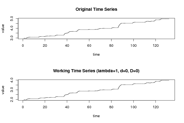
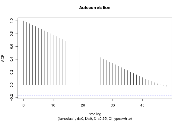
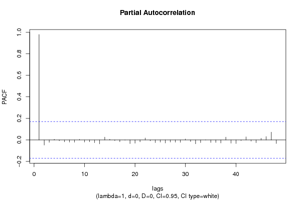
Title produced by software

(Partial) Autocorrelation Function

Date of computation

Wed, 23 Nov 2011 07:58:30 -0500

Cite this page as follows

Statistical Computations at FreeStatistics.org, Office for Research Development and Education, URL https://freestatistics.org/blog/index.php?v=date/2011/Nov/23/t13220532153iiwn4yvyvnopgy.htm/, Retrieved Fri, 26 Apr 2024 11:15:29 +0000

Statistical Computations at FreeStatistics.org, Office for Research Development and Education, URL https://freestatistics.org/blog/index.php?pk=146502, Retrieved Fri, 26 Apr 2024 11:15:29 +0000

QR Codes:

Paste this QR Code to cite your computation.

Original text written by user:

IsPrivate?

No (this computation is public)

User-defined keywords

KDGP2W12

Estimated Impact

114

Family? (F = Feedback message, R = changed R code, M = changed R Module, P = changed Parameters, D = changed Data)

-       [(Partial) Autocorrelation Function] [] [2011-11-23 12:58:30] [ded1bbd321fb25f4a0a8bacc8426c40e] [Current]

Feedback Forum

Post a new message

Dataseries X:

Download CSV

Histogram

Boxplots

2,98
2,98
2,98
3,03
3,07
3,08
3,08
3,08
3,08
3,08
3,08
3,08
3,08
3,08
3,12
3,15
3,15
3,15
3,15
3,16
3,19
3,20
3,20
3,20
3,21
3,21
3,21
3,21
3,21
3,28
3,30
3,30
3,30
3,30
3,30
3,30
3,30
3,45
3,49
3,50
3,54
3,64
3,67
3,67
3,68
3,68
3,68
3,68
3,70
3,83
3,87
3,87
3,87
3,87
3,87
3,87
3,87
3,87
3,87
3,88
3,88
3,88
3,88
3,88
3,88
3,89
3,89
3,91
3,95
3,99
3,99
3,99
4,00
4,00
4,00
4,00
4,00
4,00
4,00
4,00
4,06
4,07
4,07
4,07
4,07
4,07
4,30
4,44
4,52
4,52
4,52
4,53
4,53
4,53
4,53
4,53
4,53
4,53
4,53
4,61
4,63
4,63
4,63
4,63
4,63
4,63
4,63
4,63
4,63
4,63
4,66
4,73
4,73
4,72
4,7
4,74
4,74
4,74
4,76
4,88
4,88
4,88
4,88
4,89
4,97
4,97
4,97
4,97
4,97
4,97
4,97
4,97

Summary of computational transaction
Raw Input	view raw input (R code)
Raw Output	view raw output of R engine
Computing time	2 seconds
R Server	'Gertrude Mary Cox' @ cox.wessa.net

\begin{tabular}{lllllllll}
\hline
Summary of computational transaction \tabularnewline
Raw Input & view raw input (R code)  \tabularnewline
Raw Output & view raw output of R engine  \tabularnewline
Computing time & 2 seconds \tabularnewline
R Server & 'Gertrude Mary Cox' @ cox.wessa.net \tabularnewline
\hline
\end{tabular}
%Source: https://freestatistics.org/blog/index.php?pk=146502&T=0

[TABLE]
[ROW][C]Summary of computational transaction[/C][/ROW]
[ROW][C]Raw Input[/C][C]view raw input (R code) [/C][/ROW]
[ROW][C]Raw Output[/C][C]view raw output of R engine [/C][/ROW]
[ROW][C]Computing time[/C][C]2 seconds[/C][/ROW]
[ROW][C]R Server[/C][C]'Gertrude Mary Cox' @ cox.wessa.net[/C][/ROW]
[/TABLE]
Source: https://freestatistics.org/blog/index.php?pk=146502&T=0

Globally Unique Identifier (entire table): ba.freestatistics.org/blog/index.php?pk=146502&T=0

As an alternative you can also use a QR Code:

The GUIDs for individual cells are displayed in the table below:

Summary of computational transaction
Raw Input	view raw input (R code)
Raw Output	view raw output of R engine
Computing time	2 seconds
R Server	'Gertrude Mary Cox' @ cox.wessa.net

Autocorrelation Function
Time lag k	ACF(k)	T-STAT	P-value
1	0.979253	11.2508	0
2	0.956979	10.9949	0
3	0.934222	10.7334	0
4	0.912168	10.48	0
5	0.890336	10.2292	0
6	0.868286	9.9759	0
7	0.845878	9.7184	0
8	0.823058	9.4562	0
9	0.800969	9.2024	0
10	0.778631	8.9458	0
11	0.756113	8.6871	0
12	0.733033	8.4219	0
13	0.708957	8.1453	0
14	0.686474	7.887	0
15	0.664912	7.6393	0
16	0.643784	7.3965	0
17	0.622467	7.1516	0
18	0.601575	6.9116	0
19	0.579814	6.6616	0
20	0.557366	6.4036	0
21	0.534784	6.1442	0
22	0.5135	5.8997	0
23	0.492556	5.659	0
24	0.471224	5.4139	0
25	0.449611	5.1656	0
26	0.427443	4.9109	1e-06
27	0.40509	4.6541	4e-06
28	0.382471	4.3943	1.1e-05
29	0.359579	4.1312	3.2e-05
30	0.337647	3.8793	8.2e-05
31	0.315734	3.6275	0.000204
32	0.293099	3.3674	0.000497
33	0.270195	3.1043	0.001167
34	0.248165	2.8512	0.002528
35	0.225862	2.595	0.005265
36	0.203284	2.3356	0.010511
37	0.180266	2.0711	0.020149
38	0.158978	1.8265	0.035016
39	0.137341	1.5779	0.058488
40	0.115262	1.3243	0.093853
41	0.093755	1.0772	0.141686
42	0.074246	0.853	0.197597
43	0.055101	0.6331	0.263893
44	0.035627	0.4093	0.341485
45	0.017544	0.2016	0.420282
46	0.001521	0.0175	0.49304
47	-0.010729	-0.1233	0.45104
48	-0.023389	-0.2687	0.394282

\begin{tabular}{lllllllll}
\hline
Autocorrelation Function \tabularnewline
Time lag k & ACF(k) & T-STAT & P-value \tabularnewline
1 & 0.979253 & 11.2508 & 0 \tabularnewline
2 & 0.956979 & 10.9949 & 0 \tabularnewline
3 & 0.934222 & 10.7334 & 0 \tabularnewline
4 & 0.912168 & 10.48 & 0 \tabularnewline
5 & 0.890336 & 10.2292 & 0 \tabularnewline
6 & 0.868286 & 9.9759 & 0 \tabularnewline
7 & 0.845878 & 9.7184 & 0 \tabularnewline
8 & 0.823058 & 9.4562 & 0 \tabularnewline
9 & 0.800969 & 9.2024 & 0 \tabularnewline
10 & 0.778631 & 8.9458 & 0 \tabularnewline
11 & 0.756113 & 8.6871 & 0 \tabularnewline
12 & 0.733033 & 8.4219 & 0 \tabularnewline
13 & 0.708957 & 8.1453 & 0 \tabularnewline
14 & 0.686474 & 7.887 & 0 \tabularnewline
15 & 0.664912 & 7.6393 & 0 \tabularnewline
16 & 0.643784 & 7.3965 & 0 \tabularnewline
17 & 0.622467 & 7.1516 & 0 \tabularnewline
18 & 0.601575 & 6.9116 & 0 \tabularnewline
19 & 0.579814 & 6.6616 & 0 \tabularnewline
20 & 0.557366 & 6.4036 & 0 \tabularnewline
21 & 0.534784 & 6.1442 & 0 \tabularnewline
22 & 0.5135 & 5.8997 & 0 \tabularnewline
23 & 0.492556 & 5.659 & 0 \tabularnewline
24 & 0.471224 & 5.4139 & 0 \tabularnewline
25 & 0.449611 & 5.1656 & 0 \tabularnewline
26 & 0.427443 & 4.9109 & 1e-06 \tabularnewline
27 & 0.40509 & 4.6541 & 4e-06 \tabularnewline
28 & 0.382471 & 4.3943 & 1.1e-05 \tabularnewline
29 & 0.359579 & 4.1312 & 3.2e-05 \tabularnewline
30 & 0.337647 & 3.8793 & 8.2e-05 \tabularnewline
31 & 0.315734 & 3.6275 & 0.000204 \tabularnewline
32 & 0.293099 & 3.3674 & 0.000497 \tabularnewline
33 & 0.270195 & 3.1043 & 0.001167 \tabularnewline
34 & 0.248165 & 2.8512 & 0.002528 \tabularnewline
35 & 0.225862 & 2.595 & 0.005265 \tabularnewline
36 & 0.203284 & 2.3356 & 0.010511 \tabularnewline
37 & 0.180266 & 2.0711 & 0.020149 \tabularnewline
38 & 0.158978 & 1.8265 & 0.035016 \tabularnewline
39 & 0.137341 & 1.5779 & 0.058488 \tabularnewline
40 & 0.115262 & 1.3243 & 0.093853 \tabularnewline
41 & 0.093755 & 1.0772 & 0.141686 \tabularnewline
42 & 0.074246 & 0.853 & 0.197597 \tabularnewline
43 & 0.055101 & 0.6331 & 0.263893 \tabularnewline
44 & 0.035627 & 0.4093 & 0.341485 \tabularnewline
45 & 0.017544 & 0.2016 & 0.420282 \tabularnewline
46 & 0.001521 & 0.0175 & 0.49304 \tabularnewline
47 & -0.010729 & -0.1233 & 0.45104 \tabularnewline
48 & -0.023389 & -0.2687 & 0.394282 \tabularnewline
\hline
\end{tabular}
%Source: https://freestatistics.org/blog/index.php?pk=146502&T=1

[TABLE]
[ROW][C]Autocorrelation Function[/C][/ROW]
[ROW][C]Time lag k[/C][C]ACF(k)[/C][C]T-STAT[/C][C]P-value[/C][/ROW]
[ROW][C]1[/C][C]0.979253[/C][C]11.2508[/C][C]0[/C][/ROW]
[ROW][C]2[/C][C]0.956979[/C][C]10.9949[/C][C]0[/C][/ROW]
[ROW][C]3[/C][C]0.934222[/C][C]10.7334[/C][C]0[/C][/ROW]
[ROW][C]4[/C][C]0.912168[/C][C]10.48[/C][C]0[/C][/ROW]
[ROW][C]5[/C][C]0.890336[/C][C]10.2292[/C][C]0[/C][/ROW]
[ROW][C]6[/C][C]0.868286[/C][C]9.9759[/C][C]0[/C][/ROW]
[ROW][C]7[/C][C]0.845878[/C][C]9.7184[/C][C]0[/C][/ROW]
[ROW][C]8[/C][C]0.823058[/C][C]9.4562[/C][C]0[/C][/ROW]
[ROW][C]9[/C][C]0.800969[/C][C]9.2024[/C][C]0[/C][/ROW]
[ROW][C]10[/C][C]0.778631[/C][C]8.9458[/C][C]0[/C][/ROW]
[ROW][C]11[/C][C]0.756113[/C][C]8.6871[/C][C]0[/C][/ROW]
[ROW][C]12[/C][C]0.733033[/C][C]8.4219[/C][C]0[/C][/ROW]
[ROW][C]13[/C][C]0.708957[/C][C]8.1453[/C][C]0[/C][/ROW]
[ROW][C]14[/C][C]0.686474[/C][C]7.887[/C][C]0[/C][/ROW]
[ROW][C]15[/C][C]0.664912[/C][C]7.6393[/C][C]0[/C][/ROW]
[ROW][C]16[/C][C]0.643784[/C][C]7.3965[/C][C]0[/C][/ROW]
[ROW][C]17[/C][C]0.622467[/C][C]7.1516[/C][C]0[/C][/ROW]
[ROW][C]18[/C][C]0.601575[/C][C]6.9116[/C][C]0[/C][/ROW]
[ROW][C]19[/C][C]0.579814[/C][C]6.6616[/C][C]0[/C][/ROW]
[ROW][C]20[/C][C]0.557366[/C][C]6.4036[/C][C]0[/C][/ROW]
[ROW][C]21[/C][C]0.534784[/C][C]6.1442[/C][C]0[/C][/ROW]
[ROW][C]22[/C][C]0.5135[/C][C]5.8997[/C][C]0[/C][/ROW]
[ROW][C]23[/C][C]0.492556[/C][C]5.659[/C][C]0[/C][/ROW]
[ROW][C]24[/C][C]0.471224[/C][C]5.4139[/C][C]0[/C][/ROW]
[ROW][C]25[/C][C]0.449611[/C][C]5.1656[/C][C]0[/C][/ROW]
[ROW][C]26[/C][C]0.427443[/C][C]4.9109[/C][C]1e-06[/C][/ROW]
[ROW][C]27[/C][C]0.40509[/C][C]4.6541[/C][C]4e-06[/C][/ROW]
[ROW][C]28[/C][C]0.382471[/C][C]4.3943[/C][C]1.1e-05[/C][/ROW]
[ROW][C]29[/C][C]0.359579[/C][C]4.1312[/C][C]3.2e-05[/C][/ROW]
[ROW][C]30[/C][C]0.337647[/C][C]3.8793[/C][C]8.2e-05[/C][/ROW]
[ROW][C]31[/C][C]0.315734[/C][C]3.6275[/C][C]0.000204[/C][/ROW]
[ROW][C]32[/C][C]0.293099[/C][C]3.3674[/C][C]0.000497[/C][/ROW]
[ROW][C]33[/C][C]0.270195[/C][C]3.1043[/C][C]0.001167[/C][/ROW]
[ROW][C]34[/C][C]0.248165[/C][C]2.8512[/C][C]0.002528[/C][/ROW]
[ROW][C]35[/C][C]0.225862[/C][C]2.595[/C][C]0.005265[/C][/ROW]
[ROW][C]36[/C][C]0.203284[/C][C]2.3356[/C][C]0.010511[/C][/ROW]
[ROW][C]37[/C][C]0.180266[/C][C]2.0711[/C][C]0.020149[/C][/ROW]
[ROW][C]38[/C][C]0.158978[/C][C]1.8265[/C][C]0.035016[/C][/ROW]
[ROW][C]39[/C][C]0.137341[/C][C]1.5779[/C][C]0.058488[/C][/ROW]
[ROW][C]40[/C][C]0.115262[/C][C]1.3243[/C][C]0.093853[/C][/ROW]
[ROW][C]41[/C][C]0.093755[/C][C]1.0772[/C][C]0.141686[/C][/ROW]
[ROW][C]42[/C][C]0.074246[/C][C]0.853[/C][C]0.197597[/C][/ROW]
[ROW][C]43[/C][C]0.055101[/C][C]0.6331[/C][C]0.263893[/C][/ROW]
[ROW][C]44[/C][C]0.035627[/C][C]0.4093[/C][C]0.341485[/C][/ROW]
[ROW][C]45[/C][C]0.017544[/C][C]0.2016[/C][C]0.420282[/C][/ROW]
[ROW][C]46[/C][C]0.001521[/C][C]0.0175[/C][C]0.49304[/C][/ROW]
[ROW][C]47[/C][C]-0.010729[/C][C]-0.1233[/C][C]0.45104[/C][/ROW]
[ROW][C]48[/C][C]-0.023389[/C][C]-0.2687[/C][C]0.394282[/C][/ROW]
[/TABLE]
Source: https://freestatistics.org/blog/index.php?pk=146502&T=1

Globally Unique Identifier (entire table): ba.freestatistics.org/blog/index.php?pk=146502&T=1

As an alternative you can also use a QR Code:

The GUIDs for individual cells are displayed in the table below:

Autocorrelation Function
Time lag k	ACF(k)	T-STAT	P-value
1	0.979253	11.2508	0
2	0.956979	10.9949	0
3	0.934222	10.7334	0
4	0.912168	10.48	0
5	0.890336	10.2292	0
6	0.868286	9.9759	0
7	0.845878	9.7184	0
8	0.823058	9.4562	0
9	0.800969	9.2024	0
10	0.778631	8.9458	0
11	0.756113	8.6871	0
12	0.733033	8.4219	0
13	0.708957	8.1453	0
14	0.686474	7.887	0
15	0.664912	7.6393	0
16	0.643784	7.3965	0
17	0.622467	7.1516	0
18	0.601575	6.9116	0
19	0.579814	6.6616	0
20	0.557366	6.4036	0
21	0.534784	6.1442	0
22	0.5135	5.8997	0
23	0.492556	5.659	0
24	0.471224	5.4139	0
25	0.449611	5.1656	0
26	0.427443	4.9109	1e-06
27	0.40509	4.6541	4e-06
28	0.382471	4.3943	1.1e-05
29	0.359579	4.1312	3.2e-05
30	0.337647	3.8793	8.2e-05
31	0.315734	3.6275	0.000204
32	0.293099	3.3674	0.000497
33	0.270195	3.1043	0.001167
34	0.248165	2.8512	0.002528
35	0.225862	2.595	0.005265
36	0.203284	2.3356	0.010511
37	0.180266	2.0711	0.020149
38	0.158978	1.8265	0.035016
39	0.137341	1.5779	0.058488
40	0.115262	1.3243	0.093853
41	0.093755	1.0772	0.141686
42	0.074246	0.853	0.197597
43	0.055101	0.6331	0.263893
44	0.035627	0.4093	0.341485
45	0.017544	0.2016	0.420282
46	0.001521	0.0175	0.49304
47	-0.010729	-0.1233	0.45104
48	-0.023389	-0.2687	0.394282

Partial Autocorrelation Function
Time lag k	PACF(k)	T-STAT	P-value
1	0.979253	11.2508	0
2	-0.047651	-0.5475	0.29249
3	-0.021838	-0.2509	0.401143
4	0.006173	0.0709	0.471785
5	-0.007215	-0.0829	0.467029
6	-0.017626	-0.2025	0.419916
7	-0.019983	-0.2296	0.409384
8	-0.021272	-0.2444	0.40365
9	0.006047	0.0695	0.472356
10	-0.01974	-0.2268	0.410465
11	-0.017322	-0.199	0.421279
12	-0.025474	-0.2927	0.385114
13	-0.036515	-0.4195	0.337756
14	0.026656	0.3062	0.379949
15	0.006344	0.0729	0.471003
16	-0.005921	-0.068	0.472935
17	-0.016919	-0.1944	0.423085
18	-0.001289	-0.0148	0.494105
19	-0.034373	-0.3949	0.346772
20	-0.030216	-0.3472	0.364513
21	-0.017564	-0.2018	0.420195
22	0.018511	0.2127	0.415953
23	-0.00826	-0.0949	0.46227
24	-0.024768	-0.2846	0.388212
25	-0.020413	-0.2345	0.407469
26	-0.028704	-0.3298	0.371043
27	-0.01978	-0.2273	0.410287
28	-0.021754	-0.2499	0.401513
29	-0.022403	-0.2574	0.398638
30	0.008643	0.0993	0.460526
31	-0.015187	-0.1745	0.430874
32	-0.036041	-0.4141	0.339745
33	-0.024505	-0.2815	0.389369
34	0.001453	0.0167	0.493355
35	-0.023922	-0.2748	0.391932
36	-0.02368	-0.2721	0.393001
37	-0.028067	-0.3225	0.373804
38	0.026053	0.2993	0.382582
39	-0.030066	-0.3454	0.36516
40	-0.033422	-0.384	0.350801
41	-0.006127	-0.0704	0.471995
42	0.028669	0.3294	0.371194
43	-0.011045	-0.1269	0.449608
44	-0.025882	-0.2974	0.383328
45	0.015742	0.1809	0.428377
46	0.031649	0.3636	0.358364
47	0.072749	0.8358	0.202384
48	-0.033401	-0.3838	0.35089

\begin{tabular}{lllllllll}
\hline
Partial Autocorrelation Function \tabularnewline
Time lag k & PACF(k) & T-STAT & P-value \tabularnewline
1 & 0.979253 & 11.2508 & 0 \tabularnewline
2 & -0.047651 & -0.5475 & 0.29249 \tabularnewline
3 & -0.021838 & -0.2509 & 0.401143 \tabularnewline
4 & 0.006173 & 0.0709 & 0.471785 \tabularnewline
5 & -0.007215 & -0.0829 & 0.467029 \tabularnewline
6 & -0.017626 & -0.2025 & 0.419916 \tabularnewline
7 & -0.019983 & -0.2296 & 0.409384 \tabularnewline
8 & -0.021272 & -0.2444 & 0.40365 \tabularnewline
9 & 0.006047 & 0.0695 & 0.472356 \tabularnewline
10 & -0.01974 & -0.2268 & 0.410465 \tabularnewline
11 & -0.017322 & -0.199 & 0.421279 \tabularnewline
12 & -0.025474 & -0.2927 & 0.385114 \tabularnewline
13 & -0.036515 & -0.4195 & 0.337756 \tabularnewline
14 & 0.026656 & 0.3062 & 0.379949 \tabularnewline
15 & 0.006344 & 0.0729 & 0.471003 \tabularnewline
16 & -0.005921 & -0.068 & 0.472935 \tabularnewline
17 & -0.016919 & -0.1944 & 0.423085 \tabularnewline
18 & -0.001289 & -0.0148 & 0.494105 \tabularnewline
19 & -0.034373 & -0.3949 & 0.346772 \tabularnewline
20 & -0.030216 & -0.3472 & 0.364513 \tabularnewline
21 & -0.017564 & -0.2018 & 0.420195 \tabularnewline
22 & 0.018511 & 0.2127 & 0.415953 \tabularnewline
23 & -0.00826 & -0.0949 & 0.46227 \tabularnewline
24 & -0.024768 & -0.2846 & 0.388212 \tabularnewline
25 & -0.020413 & -0.2345 & 0.407469 \tabularnewline
26 & -0.028704 & -0.3298 & 0.371043 \tabularnewline
27 & -0.01978 & -0.2273 & 0.410287 \tabularnewline
28 & -0.021754 & -0.2499 & 0.401513 \tabularnewline
29 & -0.022403 & -0.2574 & 0.398638 \tabularnewline
30 & 0.008643 & 0.0993 & 0.460526 \tabularnewline
31 & -0.015187 & -0.1745 & 0.430874 \tabularnewline
32 & -0.036041 & -0.4141 & 0.339745 \tabularnewline
33 & -0.024505 & -0.2815 & 0.389369 \tabularnewline
34 & 0.001453 & 0.0167 & 0.493355 \tabularnewline
35 & -0.023922 & -0.2748 & 0.391932 \tabularnewline
36 & -0.02368 & -0.2721 & 0.393001 \tabularnewline
37 & -0.028067 & -0.3225 & 0.373804 \tabularnewline
38 & 0.026053 & 0.2993 & 0.382582 \tabularnewline
39 & -0.030066 & -0.3454 & 0.36516 \tabularnewline
40 & -0.033422 & -0.384 & 0.350801 \tabularnewline
41 & -0.006127 & -0.0704 & 0.471995 \tabularnewline
42 & 0.028669 & 0.3294 & 0.371194 \tabularnewline
43 & -0.011045 & -0.1269 & 0.449608 \tabularnewline
44 & -0.025882 & -0.2974 & 0.383328 \tabularnewline
45 & 0.015742 & 0.1809 & 0.428377 \tabularnewline
46 & 0.031649 & 0.3636 & 0.358364 \tabularnewline
47 & 0.072749 & 0.8358 & 0.202384 \tabularnewline
48 & -0.033401 & -0.3838 & 0.35089 \tabularnewline
\hline
\end{tabular}
%Source: https://freestatistics.org/blog/index.php?pk=146502&T=2

[TABLE]
[ROW][C]Partial Autocorrelation Function[/C][/ROW]
[ROW][C]Time lag k[/C][C]PACF(k)[/C][C]T-STAT[/C][C]P-value[/C][/ROW]
[ROW][C]1[/C][C]0.979253[/C][C]11.2508[/C][C]0[/C][/ROW]
[ROW][C]2[/C][C]-0.047651[/C][C]-0.5475[/C][C]0.29249[/C][/ROW]
[ROW][C]3[/C][C]-0.021838[/C][C]-0.2509[/C][C]0.401143[/C][/ROW]
[ROW][C]4[/C][C]0.006173[/C][C]0.0709[/C][C]0.471785[/C][/ROW]
[ROW][C]5[/C][C]-0.007215[/C][C]-0.0829[/C][C]0.467029[/C][/ROW]
[ROW][C]6[/C][C]-0.017626[/C][C]-0.2025[/C][C]0.419916[/C][/ROW]
[ROW][C]7[/C][C]-0.019983[/C][C]-0.2296[/C][C]0.409384[/C][/ROW]
[ROW][C]8[/C][C]-0.021272[/C][C]-0.2444[/C][C]0.40365[/C][/ROW]
[ROW][C]9[/C][C]0.006047[/C][C]0.0695[/C][C]0.472356[/C][/ROW]
[ROW][C]10[/C][C]-0.01974[/C][C]-0.2268[/C][C]0.410465[/C][/ROW]
[ROW][C]11[/C][C]-0.017322[/C][C]-0.199[/C][C]0.421279[/C][/ROW]
[ROW][C]12[/C][C]-0.025474[/C][C]-0.2927[/C][C]0.385114[/C][/ROW]
[ROW][C]13[/C][C]-0.036515[/C][C]-0.4195[/C][C]0.337756[/C][/ROW]
[ROW][C]14[/C][C]0.026656[/C][C]0.3062[/C][C]0.379949[/C][/ROW]
[ROW][C]15[/C][C]0.006344[/C][C]0.0729[/C][C]0.471003[/C][/ROW]
[ROW][C]16[/C][C]-0.005921[/C][C]-0.068[/C][C]0.472935[/C][/ROW]
[ROW][C]17[/C][C]-0.016919[/C][C]-0.1944[/C][C]0.423085[/C][/ROW]
[ROW][C]18[/C][C]-0.001289[/C][C]-0.0148[/C][C]0.494105[/C][/ROW]
[ROW][C]19[/C][C]-0.034373[/C][C]-0.3949[/C][C]0.346772[/C][/ROW]
[ROW][C]20[/C][C]-0.030216[/C][C]-0.3472[/C][C]0.364513[/C][/ROW]
[ROW][C]21[/C][C]-0.017564[/C][C]-0.2018[/C][C]0.420195[/C][/ROW]
[ROW][C]22[/C][C]0.018511[/C][C]0.2127[/C][C]0.415953[/C][/ROW]
[ROW][C]23[/C][C]-0.00826[/C][C]-0.0949[/C][C]0.46227[/C][/ROW]
[ROW][C]24[/C][C]-0.024768[/C][C]-0.2846[/C][C]0.388212[/C][/ROW]
[ROW][C]25[/C][C]-0.020413[/C][C]-0.2345[/C][C]0.407469[/C][/ROW]
[ROW][C]26[/C][C]-0.028704[/C][C]-0.3298[/C][C]0.371043[/C][/ROW]
[ROW][C]27[/C][C]-0.01978[/C][C]-0.2273[/C][C]0.410287[/C][/ROW]
[ROW][C]28[/C][C]-0.021754[/C][C]-0.2499[/C][C]0.401513[/C][/ROW]
[ROW][C]29[/C][C]-0.022403[/C][C]-0.2574[/C][C]0.398638[/C][/ROW]
[ROW][C]30[/C][C]0.008643[/C][C]0.0993[/C][C]0.460526[/C][/ROW]
[ROW][C]31[/C][C]-0.015187[/C][C]-0.1745[/C][C]0.430874[/C][/ROW]
[ROW][C]32[/C][C]-0.036041[/C][C]-0.4141[/C][C]0.339745[/C][/ROW]
[ROW][C]33[/C][C]-0.024505[/C][C]-0.2815[/C][C]0.389369[/C][/ROW]
[ROW][C]34[/C][C]0.001453[/C][C]0.0167[/C][C]0.493355[/C][/ROW]
[ROW][C]35[/C][C]-0.023922[/C][C]-0.2748[/C][C]0.391932[/C][/ROW]
[ROW][C]36[/C][C]-0.02368[/C][C]-0.2721[/C][C]0.393001[/C][/ROW]
[ROW][C]37[/C][C]-0.028067[/C][C]-0.3225[/C][C]0.373804[/C][/ROW]
[ROW][C]38[/C][C]0.026053[/C][C]0.2993[/C][C]0.382582[/C][/ROW]
[ROW][C]39[/C][C]-0.030066[/C][C]-0.3454[/C][C]0.36516[/C][/ROW]
[ROW][C]40[/C][C]-0.033422[/C][C]-0.384[/C][C]0.350801[/C][/ROW]
[ROW][C]41[/C][C]-0.006127[/C][C]-0.0704[/C][C]0.471995[/C][/ROW]
[ROW][C]42[/C][C]0.028669[/C][C]0.3294[/C][C]0.371194[/C][/ROW]
[ROW][C]43[/C][C]-0.011045[/C][C]-0.1269[/C][C]0.449608[/C][/ROW]
[ROW][C]44[/C][C]-0.025882[/C][C]-0.2974[/C][C]0.383328[/C][/ROW]
[ROW][C]45[/C][C]0.015742[/C][C]0.1809[/C][C]0.428377[/C][/ROW]
[ROW][C]46[/C][C]0.031649[/C][C]0.3636[/C][C]0.358364[/C][/ROW]
[ROW][C]47[/C][C]0.072749[/C][C]0.8358[/C][C]0.202384[/C][/ROW]
[ROW][C]48[/C][C]-0.033401[/C][C]-0.3838[/C][C]0.35089[/C][/ROW]
[/TABLE]
Source: https://freestatistics.org/blog/index.php?pk=146502&T=2

Globally Unique Identifier (entire table): ba.freestatistics.org/blog/index.php?pk=146502&T=2

As an alternative you can also use a QR Code:

The GUIDs for individual cells are displayed in the table below:

Partial Autocorrelation Function
Time lag k	PACF(k)	T-STAT	P-value
1	0.979253	11.2508	0
2	-0.047651	-0.5475	0.29249
3	-0.021838	-0.2509	0.401143
4	0.006173	0.0709	0.471785
5	-0.007215	-0.0829	0.467029
6	-0.017626	-0.2025	0.419916
7	-0.019983	-0.2296	0.409384
8	-0.021272	-0.2444	0.40365
9	0.006047	0.0695	0.472356
10	-0.01974	-0.2268	0.410465
11	-0.017322	-0.199	0.421279
12	-0.025474	-0.2927	0.385114
13	-0.036515	-0.4195	0.337756
14	0.026656	0.3062	0.379949
15	0.006344	0.0729	0.471003
16	-0.005921	-0.068	0.472935
17	-0.016919	-0.1944	0.423085
18	-0.001289	-0.0148	0.494105
19	-0.034373	-0.3949	0.346772
20	-0.030216	-0.3472	0.364513
21	-0.017564	-0.2018	0.420195
22	0.018511	0.2127	0.415953
23	-0.00826	-0.0949	0.46227
24	-0.024768	-0.2846	0.388212
25	-0.020413	-0.2345	0.407469
26	-0.028704	-0.3298	0.371043
27	-0.01978	-0.2273	0.410287
28	-0.021754	-0.2499	0.401513
29	-0.022403	-0.2574	0.398638
30	0.008643	0.0993	0.460526
31	-0.015187	-0.1745	0.430874
32	-0.036041	-0.4141	0.339745
33	-0.024505	-0.2815	0.389369
34	0.001453	0.0167	0.493355
35	-0.023922	-0.2748	0.391932
36	-0.02368	-0.2721	0.393001
37	-0.028067	-0.3225	0.373804
38	0.026053	0.2993	0.382582
39	-0.030066	-0.3454	0.36516
40	-0.033422	-0.384	0.350801
41	-0.006127	-0.0704	0.471995
42	0.028669	0.3294	0.371194
43	-0.011045	-0.1269	0.449608
44	-0.025882	-0.2974	0.383328
45	0.015742	0.1809	0.428377
46	0.031649	0.3636	0.358364
47	0.072749	0.8358	0.202384
48	-0.033401	-0.3838	0.35089

Figure 1

PNG link

Postscript link

PDF link

Figure 2

PNG link

Postscript link

PDF link

Figure 3

PNG link

Postscript link

PDF link

Parameters (Session):

par1 = 48 ; par2 = 1 ; par3 = 0 ; par4 = 0 ; par5 = 12 ; par6 = White Noise ; par7 = 0.95 ;

Parameters (R input):

par1 = 48 ; par2 = 1 ; par3 = 0 ; par4 = 0 ; par5 = 12 ; par6 = White Noise ; par7 = 0.95 ; par8 = ;

R code (references can be found in the software module):

if (par1 == 'Default') {
par1 = 10*log10(length(x))
} else {
par1 <- as.numeric(par1)
}
par2 <- as.numeric(par2)
par3 <- as.numeric(par3)
par4 <- as.numeric(par4)
par5 <- as.numeric(par5)
if (par6 == 'White Noise') par6 <- 'white' else par6 <- 'ma'
par7 <- as.numeric(par7)
if (par8 != '') par8 <- as.numeric(par8)
ox <- x
if (par8 == '') {
if (par2 == 0) {
x <- log(x)
} else {
x <- (x ^ par2 - 1) / par2
}
} else {
x <- log(x,base=par8)
}
if (par3 > 0) x <- diff(x,lag=1,difference=par3)
if (par4 > 0) x <- diff(x,lag=par5,difference=par4)
bitmap(file='picts.png')
op <- par(mfrow=c(2,1))
plot(ox,type='l',main='Original Time Series',xlab='time',ylab='value')
if (par8=='') {
mytitle <- paste('Working Time Series (lambda=',par2,', d=',par3,', D=',par4,')',sep='')
mysub <- paste('(lambda=',par2,', d=',par3,', D=',par4,', CI=', par7, ', CI type=',par6,')',sep='')
} else {
mytitle <- paste('Working Time Series (base=',par8,', d=',par3,', D=',par4,')',sep='')
mysub <- paste('(base=',par8,', d=',par3,', D=',par4,', CI=', par7, ', CI type=',par6,')',sep='')
}
plot(x,type='l', main=mytitle,xlab='time',ylab='value')
par(op)
dev.off()
bitmap(file='pic1.png')
racf <- acf(x, par1, main='Autocorrelation', xlab='time lag', ylab='ACF', ci.type=par6, ci=par7, sub=mysub)
dev.off()
bitmap(file='pic2.png')
rpacf <- pacf(x,par1,main='Partial Autocorrelation',xlab='lags',ylab='PACF',sub=mysub)
dev.off()
(myacf <- c(racf$acf))
(mypacf <- c(rpacf$acf))
lengthx <- length(x)
sqrtn <- sqrt(lengthx)
load(file='createtable')
a<-table.start()
a<-table.row.start(a)
a<-table.element(a,'Autocorrelation Function',4,TRUE)
a<-table.row.end(a)
a<-table.row.start(a)
a<-table.element(a,'Time lag k',header=TRUE)
a<-table.element(a,hyperlink('basics.htm','ACF(k)','click here for more information about the Autocorrelation Function'),header=TRUE)
a<-table.element(a,'T-STAT',header=TRUE)
a<-table.element(a,'P-value',header=TRUE)
a<-table.row.end(a)
for (i in 2:(par1+1)) {
a<-table.row.start(a)
a<-table.element(a,i-1,header=TRUE)
a<-table.element(a,round(myacf[i],6))
mytstat <- myacf[i]*sqrtn
a<-table.element(a,round(mytstat,4))
a<-table.element(a,round(1-pt(abs(mytstat),lengthx),6))
a<-table.row.end(a)
}
a<-table.end(a)
table.save(a,file='mytable.tab')
a<-table.start()
a<-table.row.start(a)
a<-table.element(a,'Partial Autocorrelation Function',4,TRUE)
a<-table.row.end(a)
a<-table.row.start(a)
a<-table.element(a,'Time lag k',header=TRUE)
a<-table.element(a,hyperlink('basics.htm','PACF(k)','click here for more information about the Partial Autocorrelation Function'),header=TRUE)
a<-table.element(a,'T-STAT',header=TRUE)
a<-table.element(a,'P-value',header=TRUE)
a<-table.row.end(a)
for (i in 1:par1) {
a<-table.row.start(a)
a<-table.element(a,i,header=TRUE)
a<-table.element(a,round(mypacf[i],6))
mytstat <- mypacf[i]*sqrtn
a<-table.element(a,round(mytstat,4))
a<-table.element(a,round(1-pt(abs(mytstat),lengthx),6))
a<-table.row.end(a)
}
a<-table.end(a)
table.save(a,file='mytable1.tab')

Free Statistics

Description of Statistical Computation

Tree of Dependent Computations

Dataset

Tables (Output of Computation)

Figures (Output of Computation)

Input Parameters & R Code