| Multiple Linear Regression - Estimated Regression Equation |
| huwelijk[t] = + 25.8123828175966 + 2.33103196284986sterfte[t] + 0.00250498731782159Unemployment[t] + 1.41522775733092M1[t] + 0.578603287663617M2[t] + 0.774202748962213M3[t] + 0.350550929587069M4[t] + 0.234579853787061M5[t] + 1.38601933067036M6[t] -0.00668225300051042M7[t] + 0.230707444492079M8[t] + 0.534236519164191M9[t] + 2.0930846324962M10[t] + 0.94347653748373M11[t] + e[t] |
| Multiple Linear Regression - Ordinary Least Squares | |||||
| Variable | Parameter | S.D. | T-STAT H0: parameter = 0 | 2-tail p-value | 1-tail p-value |
| (Intercept) | 25.8123828175966 | 4.198349 | 6.1482 | 1e-06 | 0 |
| sterfte | 2.33103196284986 | 0.195096 | 11.9481 | 0 | 0 |
| Unemployment | 0.00250498731782159 | 0.002264 | 1.1062 | 0.276874 | 0.138437 |
| M1 | 1.41522775733092 | 1.204476 | 1.175 | 0.248674 | 0.124337 |
| M2 | 0.578603287663617 | 1.205288 | 0.4801 | 0.634454 | 0.317227 |
| M3 | 0.774202748962213 | 1.206702 | 0.6416 | 0.525711 | 0.262856 |
| M4 | 0.350550929587069 | 1.213113 | 0.289 | 0.77447 | 0.387235 |
| M5 | 0.234579853787061 | 1.229633 | 0.1908 | 0.849909 | 0.424955 |
| M6 | 1.38601933067036 | 1.242755 | 1.1153 | 0.273036 | 0.136518 |
| M7 | -0.00668225300051042 | 1.246101 | -0.0054 | 0.995755 | 0.497877 |
| M8 | 0.230707444492079 | 1.249274 | 0.1847 | 0.854651 | 0.427325 |
| M9 | 0.534236519164191 | 1.243349 | 0.4297 | 0.670311 | 0.335156 |
| M10 | 2.0930846324962 | 1.243794 | 1.6828 | 0.102143 | 0.051072 |
| M11 | 0.94347653748373 | 1.3138 | 0.7181 | 0.477889 | 0.238945 |
| Multiple Linear Regression - Regression Statistics | |
| Multiple R | 0.961989452304715 |
| R-squared | 0.925423706345525 |
| Adjusted R-squared | 0.895127087048394 |
| F-TEST (value) | 30.5454446012455 |
| F-TEST (DF numerator) | 13 |
| F-TEST (DF denominator) | 32 |
| p-value | 2.43138842392909e-14 |
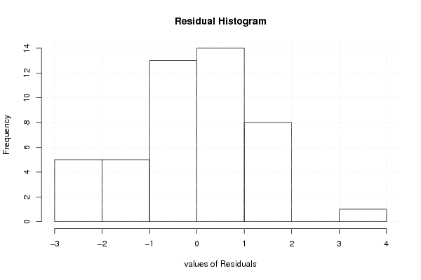
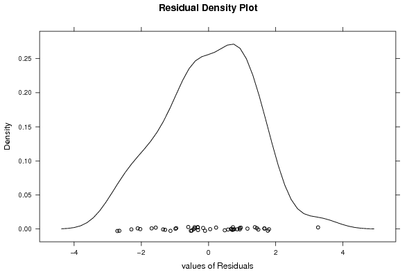
| Multiple Linear Regression - Residual Statistics | |
| Residual Standard Deviation | 1.57235150297064 |
| Sum Squared Residuals | 79.1132559646094 |
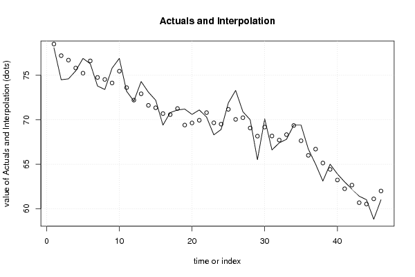
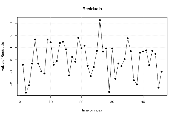
| Multiple Linear Regression - Actuals, Interpolation, and Residuals | |||
| Time or Index | Actuals | Interpolation Forecast | Residuals Prediction Error |
| 1 | 78.1 | 78.5148227347965 | -0.41482273479654 |
| 2 | 74.5 | 77.2119918725592 | -2.71199187255923 |
| 3 | 74.6 | 76.7082817450029 | -2.10828174500288 |
| 4 | 75.5 | 75.8184235330578 | -0.318423533057753 |
| 5 | 76.9 | 75.2362460646878 | 1.66375393531223 |
| 6 | 76.3 | 76.620788737856 | -0.320788737856057 |
| 7 | 73.8 | 74.7618807616152 | -0.961880761615217 |
| 8 | 73.4 | 74.5330640665378 | -1.13306406653783 |
| 9 | 75.8 | 74.137283552355 | 1.66271644764501 |
| 10 | 76.9 | 75.463028469402 | 1.436971530598 |
| 11 | 73.2 | 73.6141107855346 | -0.414110785534579 |
| 12 | 72.1 | 72.2044278554809 | -0.104427855480878 |
| 13 | 74.3 | 72.9203460239568 | 1.37965397604316 |
| 14 | 73.1 | 71.6175151617196 | 1.48248483828043 |
| 15 | 72.2 | 71.3469082304482 | 0.853091769551818 |
| 16 | 69.4 | 70.690153214788 | -1.29015321478805 |
| 17 | 70.8 | 70.574182138988 | 0.225817861011946 |
| 18 | 71.1 | 71.2594152233014 | -0.159415223301376 |
| 19 | 71.2 | 69.4005072470605 | 1.79949275293947 |
| 20 | 70.6 | 69.6378969445531 | 0.962103055446874 |
| 21 | 71.1 | 69.9414260192252 | 1.15857398077476 |
| 22 | 70.3 | 70.8009645437023 | -0.500964543702281 |
| 23 | 68.3 | 69.6513564486898 | -1.35135644868981 |
| 24 | 68.9 | 69.5030740088869 | -0.603074008886856 |
| 25 | 71.9 | 71.1714448610453 | 0.728555138954675 |
| 26 | 73.3 | 70.0395935096111 | 3.26040649038892 |
| 27 | 70.9 | 70.2266760140291 | 0.673323985970927 |
| 28 | 70 | 69.0698972770084 | 0.930102722991618 |
| 29 | 65.5 | 68.1546676183723 | -2.65466761837233 |
| 30 | 70.1 | 69.1735932661429 | 0.926406733857125 |
| 31 | 66.6 | 68.1706959618484 | -1.57069596184842 |
| 32 | 67.4 | 67.7115315565356 | -0.311531556535648 |
| 33 | 67.8 | 68.3250669381499 | -0.525066938149872 |
| 34 | 69.4 | 69.3519386154574 | 0.0480613845426075 |
| 35 | 69.4 | 67.6345327657756 | 1.76546723422439 |
| 36 | 66.7 | 65.9924981356323 | 0.707501864367734 |
| 37 | 65 | 66.6933863802013 | -1.69338638020129 |
| 38 | 63.1 | 65.1308994561101 | -2.03089945611013 |
| 39 | 65 | 64.4181340105199 | 0.58186598948013 |
| 40 | 63.9 | 63.2215259751458 | 0.678474024854189 |
| 41 | 63 | 62.2349041779518 | 0.765095822048155 |
| 42 | 62.2 | 62.6462027726997 | -0.446202772699692 |
| 43 | 61.4 | 60.6669160294758 | 0.733083970524162 |
| 44 | 61 | 60.5175074323734 | 0.4824925676266 |
| 45 | 58.8 | 61.0962234902699 | -2.2962234902699 |
| 46 | 61 | 61.9840683714383 | -0.98406837143833 |
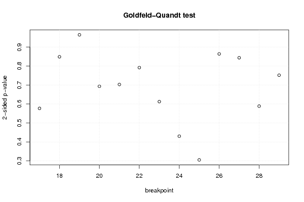
| Goldfeld-Quandt test for Heteroskedasticity | |||
| p-values | Alternative Hypothesis | ||
| breakpoint index | greater | 2-sided | less |
| 17 | 0.711453048202981 | 0.577093903594038 | 0.288546951797019 |
| 18 | 0.575663227929577 | 0.848673544140846 | 0.424336772070423 |
| 19 | 0.482248177727651 | 0.964496355455301 | 0.517751822272349 |
| 20 | 0.346629717736967 | 0.693259435473933 | 0.653370282263034 |
| 21 | 0.351385664432613 | 0.702771328865227 | 0.648614335567387 |
| 22 | 0.395904200020054 | 0.791808400040108 | 0.604095799979946 |
| 23 | 0.30628339334597 | 0.61256678669194 | 0.69371660665403 |
| 24 | 0.215261213215737 | 0.430522426431473 | 0.784738786784263 |
| 25 | 0.152777174116269 | 0.305554348232538 | 0.847222825883731 |
| 26 | 0.568066171022947 | 0.863867657954107 | 0.431933828977053 |
| 27 | 0.421783608003101 | 0.843567216006202 | 0.578216391996899 |
| 28 | 0.29441014973985 | 0.5888202994797 | 0.70558985026015 |
| 29 | 0.624115670181828 | 0.751768659636345 | 0.375884329818172 |
| Meta Analysis of Goldfeld-Quandt test for Heteroskedasticity | |||
| Description | # significant tests | % significant tests | OK/NOK |
| 1% type I error level | 0 | 0 | OK |
| 5% type I error level | 0 | 0 | OK |
| 10% type I error level | 0 | 0 | OK |