Free Statistics
of Irreproducible Research!
Description of Statistical Computation | |||||||||||||||||||||||||||||||||||||||||||||||||||||||||||||
|---|---|---|---|---|---|---|---|---|---|---|---|---|---|---|---|---|---|---|---|---|---|---|---|---|---|---|---|---|---|---|---|---|---|---|---|---|---|---|---|---|---|---|---|---|---|---|---|---|---|---|---|---|---|---|---|---|---|---|---|---|---|
| Author's title | |||||||||||||||||||||||||||||||||||||||||||||||||||||||||||||
| Author | *The author of this computation has been verified* | ||||||||||||||||||||||||||||||||||||||||||||||||||||||||||||
| R Software Module | rwasp_linear_regression.wasp | ||||||||||||||||||||||||||||||||||||||||||||||||||||||||||||
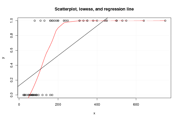
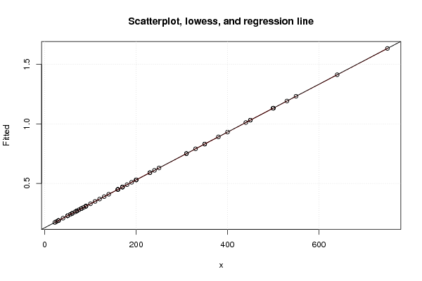
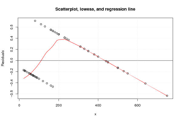
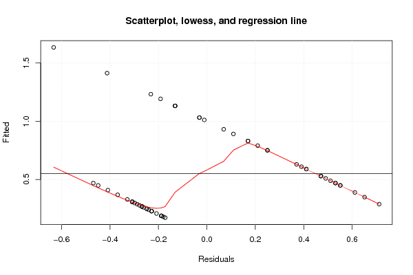
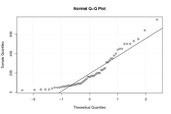
| Title produced by software | Linear Regression Graphical Model Validation | ||||||||||||||||||||||||||||||||||||||||||||||||||||||||||||
| Date of computation | Mon, 21 Nov 2011 13:27:17 -0500 | ||||||||||||||||||||||||||||||||||||||||||||||||||||||||||||
| Cite this page as follows | Statistical Computations at FreeStatistics.org, Office for Research Development and Education, URL https://freestatistics.org/blog/index.php?v=date/2011/Nov/21/t1321900057t3sagv5fsafqmi5.htm/, Retrieved Thu, 25 Apr 2024 00:48:17 +0000 | ||||||||||||||||||||||||||||||||||||||||||||||||||||||||||||
| Statistical Computations at FreeStatistics.org, Office for Research Development and Education, URL https://freestatistics.org/blog/index.php?pk=145894, Retrieved Thu, 25 Apr 2024 00:48:17 +0000 | |||||||||||||||||||||||||||||||||||||||||||||||||||||||||||||
| QR Codes: | |||||||||||||||||||||||||||||||||||||||||||||||||||||||||||||
|
| |||||||||||||||||||||||||||||||||||||||||||||||||||||||||||||
| Original text written by user: | |||||||||||||||||||||||||||||||||||||||||||||||||||||||||||||
| IsPrivate? | No (this computation is public) | ||||||||||||||||||||||||||||||||||||||||||||||||||||||||||||
| User-defined keywords | |||||||||||||||||||||||||||||||||||||||||||||||||||||||||||||
| Estimated Impact | 91 | ||||||||||||||||||||||||||||||||||||||||||||||||||||||||||||
Tree of Dependent Computations | |||||||||||||||||||||||||||||||||||||||||||||||||||||||||||||
| Family? (F = Feedback message, R = changed R code, M = changed R Module, P = changed Parameters, D = changed Data) | |||||||||||||||||||||||||||||||||||||||||||||||||||||||||||||
| - [Linear Regression Graphical Model Validation] [Colombia Coffee -...] [2008-02-26 10:22:06] [74be16979710d4c4e7c6647856088456] - RM D [Linear Regression Graphical Model Validation] [] [2011-11-21 18:23:29] [0fa8c500575976cf9d2f7efbe256ddfb] - D [Linear Regression Graphical Model Validation] [] [2011-11-21 18:24:55] [0fa8c500575976cf9d2f7efbe256ddfb] - D [Linear Regression Graphical Model Validation] [] [2011-11-21 18:27:17] [2e63149daec6ba44c7d6fab36a0b0c34] [Current] | |||||||||||||||||||||||||||||||||||||||||||||||||||||||||||||
| Feedback Forum | |||||||||||||||||||||||||||||||||||||||||||||||||||||||||||||
Post a new message | |||||||||||||||||||||||||||||||||||||||||||||||||||||||||||||
Dataset | |||||||||||||||||||||||||||||||||||||||||||||||||||||||||||||
| Dataseries X: | |||||||||||||||||||||||||||||||||||||||||||||||||||||||||||||
129.99 59.99 49.99 84.99 179.99 329.99 25.99 499.99 89.99 119.99 79.99 199.99 449.99 549.99 529.99 639.99 749.99 399.99 169.99 189.99 199.99 69.99 69.99 109.99 159.99 159.99 199.99 75 349.99 439.99 309.99 379.99 349.99 169.99 239.99 229.99 69.99 99.99 29.99 39.99 21.99 499.99 29.99 29.99 49.99 49.99 55.99 59.99 79.99 139.99 159.99 169.99 229.99 249.99 309.99 499.99 65.99 89.99 89.99 449.99 | |||||||||||||||||||||||||||||||||||||||||||||||||||||||||||||
| Dataseries Y: | |||||||||||||||||||||||||||||||||||||||||||||||||||||||||||||
1 0 0 0 1 1 0 1 0 0 1 1 1 1 1 1 1 1 1 1 1 0 0 1 1 1 1 0 1 1 1 1 1 0 1 1 0 0 0 0 0 1 0 0 0 0 0 0 0 0 0 1 1 1 1 1 0 0 0 1 | |||||||||||||||||||||||||||||||||||||||||||||||||||||||||||||
Tables (Output of Computation) | |||||||||||||||||||||||||||||||||||||||||||||||||||||||||||||
| |||||||||||||||||||||||||||||||||||||||||||||||||||||||||||||
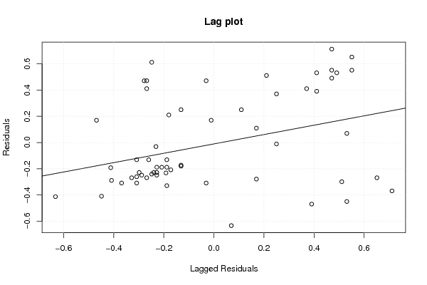
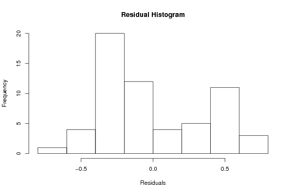
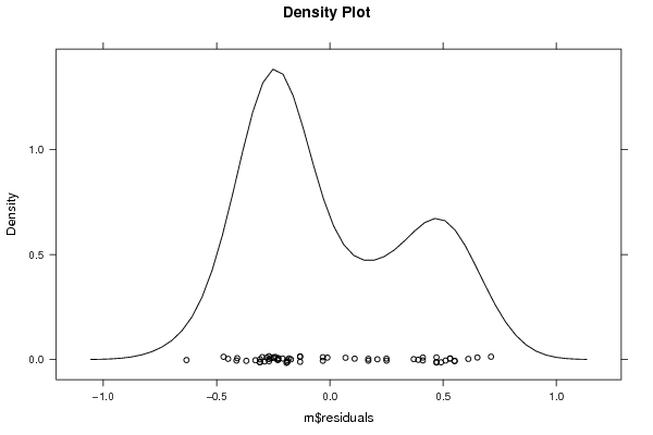
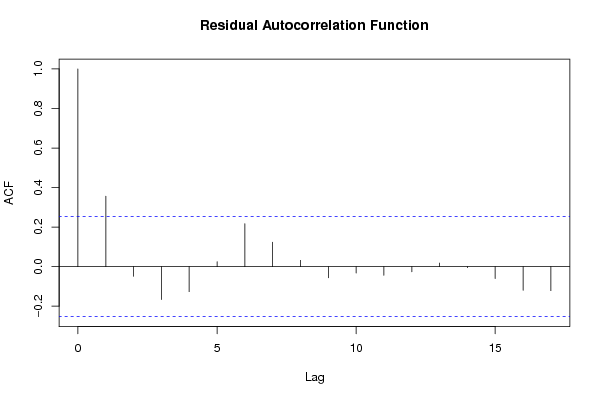
Figures (Output of Computation) | |||||||||||||||||||||||||||||||||||||||||||||||||||||||||||||
Input Parameters & R Code | |||||||||||||||||||||||||||||||||||||||||||||||||||||||||||||
| Parameters (Session): | |||||||||||||||||||||||||||||||||||||||||||||||||||||||||||||
| par1 = 0 ; | |||||||||||||||||||||||||||||||||||||||||||||||||||||||||||||
| Parameters (R input): | |||||||||||||||||||||||||||||||||||||||||||||||||||||||||||||
| par1 = 0 ; | |||||||||||||||||||||||||||||||||||||||||||||||||||||||||||||
| R code (references can be found in the software module): | |||||||||||||||||||||||||||||||||||||||||||||||||||||||||||||
par1 <- as.numeric(par1) | |||||||||||||||||||||||||||||||||||||||||||||||||||||||||||||