Free Statistics
of Irreproducible Research!
Description of Statistical Computation | |||||||||||||||||||||||||||||||||||||||||||||||||||||
|---|---|---|---|---|---|---|---|---|---|---|---|---|---|---|---|---|---|---|---|---|---|---|---|---|---|---|---|---|---|---|---|---|---|---|---|---|---|---|---|---|---|---|---|---|---|---|---|---|---|---|---|---|---|
| Author's title | |||||||||||||||||||||||||||||||||||||||||||||||||||||
| Author | *The author of this computation has been verified* | ||||||||||||||||||||||||||||||||||||||||||||||||||||
| R Software Module | rwasp_edauni.wasp | ||||||||||||||||||||||||||||||||||||||||||||||||||||
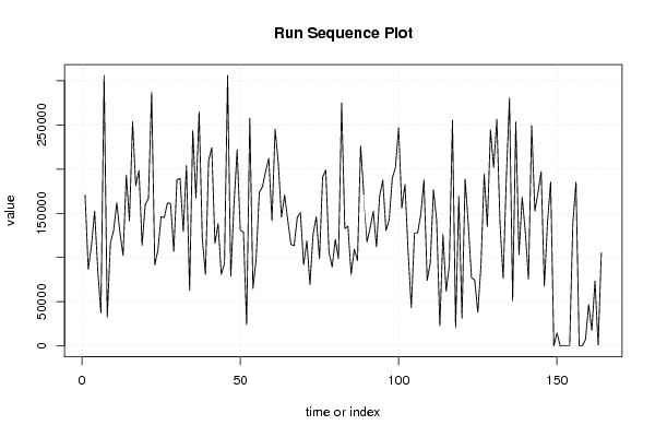
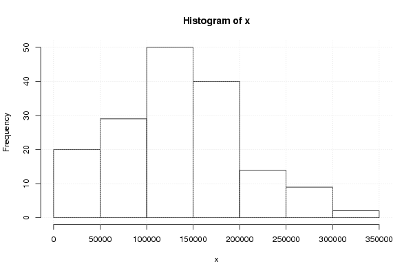
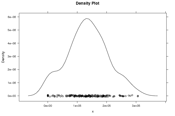
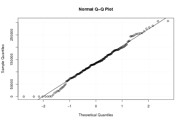
| Title produced by software | Univariate Explorative Data Analysis | ||||||||||||||||||||||||||||||||||||||||||||||||||||
| Date of computation | Mon, 21 Nov 2011 07:06:17 -0500 | ||||||||||||||||||||||||||||||||||||||||||||||||||||
| Cite this page as follows | Statistical Computations at FreeStatistics.org, Office for Research Development and Education, URL https://freestatistics.org/blog/index.php?v=date/2011/Nov/21/t1321877201yvc2py2xuilmrem.htm/, Retrieved Wed, 24 Apr 2024 17:37:25 +0000 | ||||||||||||||||||||||||||||||||||||||||||||||||||||
| Statistical Computations at FreeStatistics.org, Office for Research Development and Education, URL https://freestatistics.org/blog/index.php?pk=145714, Retrieved Wed, 24 Apr 2024 17:37:25 +0000 | |||||||||||||||||||||||||||||||||||||||||||||||||||||
| QR Codes: | |||||||||||||||||||||||||||||||||||||||||||||||||||||
|
| |||||||||||||||||||||||||||||||||||||||||||||||||||||
| Original text written by user: | |||||||||||||||||||||||||||||||||||||||||||||||||||||
| IsPrivate? | No (this computation is public) | ||||||||||||||||||||||||||||||||||||||||||||||||||||
| User-defined keywords | |||||||||||||||||||||||||||||||||||||||||||||||||||||
| Estimated Impact | 148 | ||||||||||||||||||||||||||||||||||||||||||||||||||||
Tree of Dependent Computations | |||||||||||||||||||||||||||||||||||||||||||||||||||||
| Family? (F = Feedback message, R = changed R code, M = changed R Module, P = changed Parameters, D = changed Data) | |||||||||||||||||||||||||||||||||||||||||||||||||||||
| - [Univariate Explorative Data Analysis] [time effect in su...] [2010-11-17 08:55:33] [b98453cac15ba1066b407e146608df68] - R D [Univariate Explorative Data Analysis] [WS 7 Yt Sequence ...] [2011-11-21 12:06:17] [22431204c416bf26bfe4de00cd8c0d22] [Current] - D [Univariate Explorative Data Analysis] [WS7 (2)] [2012-11-18 17:35:32] [300ac07a477d84a470eebba12c2af4b2] - RMPD [Central Tendency] [WS7 (3)] [2012-11-18 17:42:27] [300ac07a477d84a470eebba12c2af4b2] - D [Univariate Explorative Data Analysis] [Mini-Tutorial1] [2012-11-19 14:19:49] [3ba5358ad212dca7c498c7fc6d6ebde5] - D [Univariate Explorative Data Analysis] [WS7 2] [2012-11-19 16:48:58] [ec4855be6a46db5e0c29fcd049472c6d] | |||||||||||||||||||||||||||||||||||||||||||||||||||||
| Feedback Forum | |||||||||||||||||||||||||||||||||||||||||||||||||||||
Post a new message | |||||||||||||||||||||||||||||||||||||||||||||||||||||
Dataset | |||||||||||||||||||||||||||||||||||||||||||||||||||||
| Dataseries X: | |||||||||||||||||||||||||||||||||||||||||||||||||||||
170588 86621 113337 152510 86206 37257 306055 32750 116502 130539 161876 128274 102350 193024 141574 253559 181110 198432 113853 159940 166822 286675 91657 108278 146342 145142 161740 160905 106888 188150 189401 129484 204030 62731 243625 167255 264528 122024 80964 209795 224205 115971 138191 81106 93125 305756 78800 158835 221745 131108 128734 24188 257662 65029 98066 173587 180042 197266 212060 141582 245107 206879 145696 170635 142064 114820 113461 145285 150999 91812 118807 69471 126630 145908 98393 190926 198797 106193 89318 120362 98791 274953 132798 135251 80953 109237 96634 226191 171286 117815 133561 152193 112004 169613 187483 130533 142339 189764 201603 246834 155947 182581 106351 43287 127493 127930 149006 187653 74112 94006 176625 141933 22938 125927 61857 91290 255100 21054 169093 31414 188701 137544 77166 74567 38214 90961 194224 135261 244272 201748 256402 139144 76470 189502 280334 50999 253274 103239 168059 128768 75746 249232 152366 173260 197197 67507 139409 185366 0 14688 98 455 0 0 137885 185288 0 203 7199 46660 17547 73567 969 105477 | |||||||||||||||||||||||||||||||||||||||||||||||||||||
Tables (Output of Computation) | |||||||||||||||||||||||||||||||||||||||||||||||||||||
| |||||||||||||||||||||||||||||||||||||||||||||||||||||
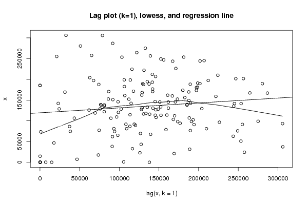
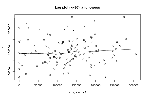
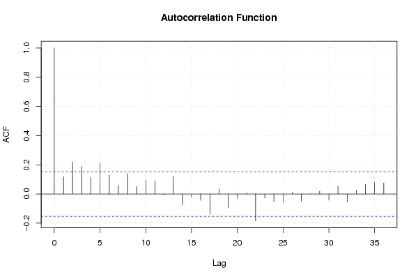
Figures (Output of Computation) | |||||||||||||||||||||||||||||||||||||||||||||||||||||
Input Parameters & R Code | |||||||||||||||||||||||||||||||||||||||||||||||||||||
| Parameters (Session): | |||||||||||||||||||||||||||||||||||||||||||||||||||||
| par1 = 0 ; par2 = 36 ; | |||||||||||||||||||||||||||||||||||||||||||||||||||||
| Parameters (R input): | |||||||||||||||||||||||||||||||||||||||||||||||||||||
| par1 = 0 ; par2 = 36 ; | |||||||||||||||||||||||||||||||||||||||||||||||||||||
| R code (references can be found in the software module): | |||||||||||||||||||||||||||||||||||||||||||||||||||||
par1 <- as.numeric(par1) | |||||||||||||||||||||||||||||||||||||||||||||||||||||