Free Statistics
of Irreproducible Research!
Description of Statistical Computation | |||||||||||||||||||||||||||||||||||||
|---|---|---|---|---|---|---|---|---|---|---|---|---|---|---|---|---|---|---|---|---|---|---|---|---|---|---|---|---|---|---|---|---|---|---|---|---|---|
| Author's title | |||||||||||||||||||||||||||||||||||||
| Author | *The author of this computation has been verified* | ||||||||||||||||||||||||||||||||||||
| R Software Module | rwasp_boxcoxnorm.wasp | ||||||||||||||||||||||||||||||||||||
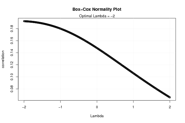
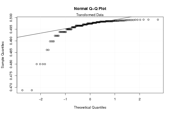
| Title produced by software | Box-Cox Normality Plot | ||||||||||||||||||||||||||||||||||||
| Date of computation | Sun, 20 Nov 2011 11:55:21 -0500 | ||||||||||||||||||||||||||||||||||||
| Cite this page as follows | Statistical Computations at FreeStatistics.org, Office for Research Development and Education, URL https://freestatistics.org/blog/index.php?v=date/2011/Nov/20/t13218081435yhjwgmatwsrk02.htm/, Retrieved Thu, 25 Apr 2024 00:17:19 +0000 | ||||||||||||||||||||||||||||||||||||
| Statistical Computations at FreeStatistics.org, Office for Research Development and Education, URL https://freestatistics.org/blog/index.php?pk=145649, Retrieved Thu, 25 Apr 2024 00:17:19 +0000 | |||||||||||||||||||||||||||||||||||||
| QR Codes: | |||||||||||||||||||||||||||||||||||||
|
| |||||||||||||||||||||||||||||||||||||
| Original text written by user: | |||||||||||||||||||||||||||||||||||||
| IsPrivate? | No (this computation is public) | ||||||||||||||||||||||||||||||||||||
| User-defined keywords | |||||||||||||||||||||||||||||||||||||
| Estimated Impact | 143 | ||||||||||||||||||||||||||||||||||||
Tree of Dependent Computations | |||||||||||||||||||||||||||||||||||||
| Family? (F = Feedback message, R = changed R code, M = changed R Module, P = changed Parameters, D = changed Data) | |||||||||||||||||||||||||||||||||||||
| - [Survey Scores] [Intrinsic Motivat...] [2010-10-12 11:18:40] [b98453cac15ba1066b407e146608df68] - R P [Survey Scores] [Intrinsic motivat...] [2011-11-20 16:09:55] [d9c77998677156eca5bd63e08beb400b] - RMPD [Maximum-likelihood Fitting - Normal Distribution] [Normale verdeling A] [2011-11-20 16:43:07] [d9c77998677156eca5bd63e08beb400b] - RM D [Box-Cox Normality Plot] [Verdeling I3] [2011-11-20 16:55:21] [8432dc408001a08517818ba7ac24bdb0] [Current] | |||||||||||||||||||||||||||||||||||||
| Feedback Forum | |||||||||||||||||||||||||||||||||||||
Post a new message | |||||||||||||||||||||||||||||||||||||
Dataset | |||||||||||||||||||||||||||||||||||||
| Dataseries X: | |||||||||||||||||||||||||||||||||||||
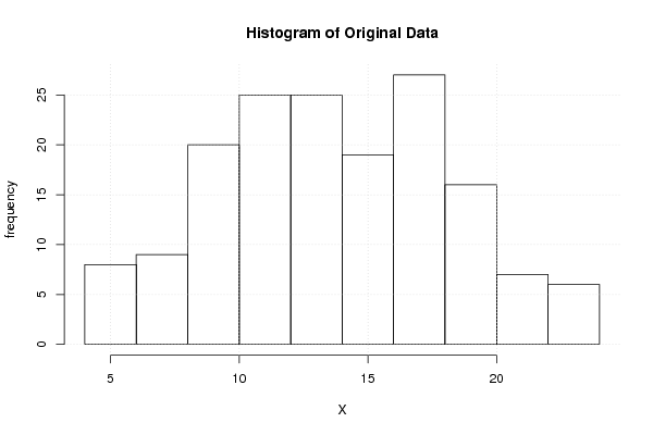
21 15 18 11 8 19 4 20 16 14 10 13 14 8 23 11 9 24 5 15 5 19 6 13 11 17 17 5 9 15 17 17 20 12 7 16 7 14 24 15 15 10 14 18 12 9 9 8 18 10 17 14 16 10 19 10 14 10 4 19 9 12 16 11 18 11 24 17 18 9 19 18 12 23 22 14 14 16 23 7 10 12 12 12 17 21 16 11 14 13 9 19 13 19 13 13 13 14 12 22 11 5 18 19 14 15 12 19 15 17 8 10 12 12 20 12 12 14 6 10 18 18 7 18 9 17 22 11 15 17 15 22 9 13 20 14 14 12 20 20 8 17 9 18 22 10 13 15 18 18 12 12 20 12 16 16 18 16 13 17 13 17 | |||||||||||||||||||||||||||||||||||||
Tables (Output of Computation) | |||||||||||||||||||||||||||||||||||||
| |||||||||||||||||||||||||||||||||||||
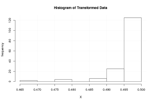
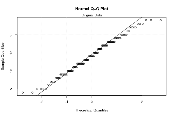
Figures (Output of Computation) | |||||||||||||||||||||||||||||||||||||
Input Parameters & R Code | |||||||||||||||||||||||||||||||||||||
| Parameters (Session): | |||||||||||||||||||||||||||||||||||||
| par1 = 8 ; par2 = 0 ; | |||||||||||||||||||||||||||||||||||||
| Parameters (R input): | |||||||||||||||||||||||||||||||||||||
| R code (references can be found in the software module): | |||||||||||||||||||||||||||||||||||||
n <- length(x) | |||||||||||||||||||||||||||||||||||||