Repository of Reproducible Computations

Free Statistics

of Irreproducible Research!

Author's title

Author

*Unverified author*

R Software Module

rwasp_autocorrelation.wasp

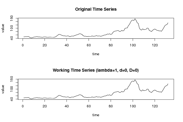
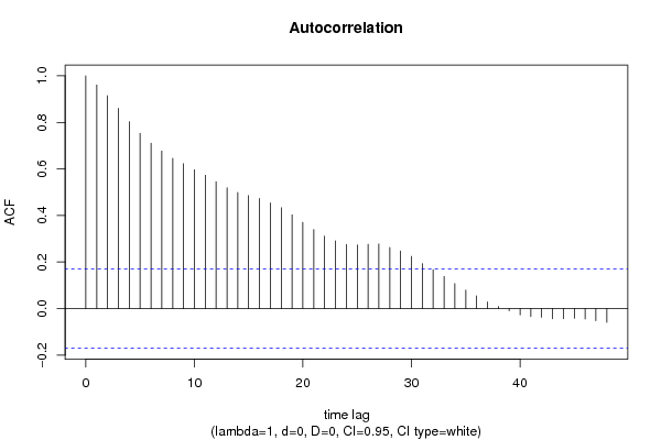
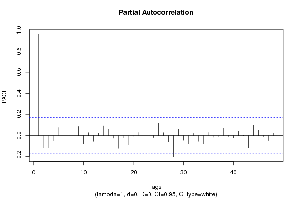
Title produced by software

(Partial) Autocorrelation Function

Date of computation

Sun, 20 Nov 2011 07:01:06 -0500

Cite this page as follows

Statistical Computations at FreeStatistics.org, Office for Research Development and Education, URL https://freestatistics.org/blog/index.php?v=date/2011/Nov/20/t1321790548zmkznsuuoeu73z8.htm/, Retrieved Tue, 23 Apr 2024 06:34:30 +0000

Statistical Computations at FreeStatistics.org, Office for Research Development and Education, URL https://freestatistics.org/blog/index.php?pk=145576, Retrieved Tue, 23 Apr 2024 06:34:30 +0000

QR Codes:

Paste this QR Code to cite your computation.

Original text written by user:

IsPrivate?

No (this computation is public)

User-defined keywords

KDGP2W12

Estimated Impact

185

Family? (F = Feedback message, R = changed R code, M = changed R Module, P = changed Parameters, D = changed Data)

-       [(Partial) Autocorrelation Function] [Opgave 6bis - ind...] [2011-11-20 12:01:06] [1dca9aa876cba4edc5cb0d742d3acdc5] [Current]

Feedback Forum

Post a new message

Dataseries X:

Download CSV

Histogram

Boxplots

Summary of computational transaction
Raw Input	view raw input (R code)
Raw Output	view raw output of R engine
Computing time	1 seconds
R Server	'Gwilym Jenkins' @ jenkins.wessa.net

\begin{tabular}{lllllllll}
\hline
Summary of computational transaction \tabularnewline
Raw Input & view raw input (R code)  \tabularnewline
Raw Output & view raw output of R engine  \tabularnewline
Computing time & 1 seconds \tabularnewline
R Server & 'Gwilym Jenkins' @ jenkins.wessa.net \tabularnewline
\hline
\end{tabular}
%Source: https://freestatistics.org/blog/index.php?pk=145576&T=0

[TABLE]
[ROW][C]Summary of computational transaction[/C][/ROW]
[ROW][C]Raw Input[/C][C]view raw input (R code) [/C][/ROW]
[ROW][C]Raw Output[/C][C]view raw output of R engine [/C][/ROW]
[ROW][C]Computing time[/C][C]1 seconds[/C][/ROW]
[ROW][C]R Server[/C][C]'Gwilym Jenkins' @ jenkins.wessa.net[/C][/ROW]
[/TABLE]
Source: https://freestatistics.org/blog/index.php?pk=145576&T=0

Globally Unique Identifier (entire table): ba.freestatistics.org/blog/index.php?pk=145576&T=0

As an alternative you can also use a QR Code:

The GUIDs for individual cells are displayed in the table below:

Summary of computational transaction
Raw Input	view raw input (R code)
Raw Output	view raw output of R engine
Computing time	1 seconds
R Server	'Gwilym Jenkins' @ jenkins.wessa.net

Autocorrelation Function
Time lag k	ACF(k)	T-STAT	P-value
1	0.961084	11.042	0
2	0.914366	10.5053	0
3	0.860047	9.8812	0
4	0.802961	9.2253	0
5	0.752843	8.6495	0
6	0.710777	8.1662	0
7	0.676603	7.7736	0
8	0.644981	7.4103	0
9	0.622473	7.1517	0
10	0.596277	6.8507	0
11	0.572569	6.5783	0
12	0.545378	6.2659	0
13	0.518749	5.96	0
14	0.49921	5.7355	0
15	0.485196	5.5745	0
16	0.473265	5.4374	0
17	0.454021	5.2163	0
18	0.433441	4.9799	1e-06
19	0.403187	4.6323	4e-06
20	0.370498	4.2567	2e-05
21	0.339144	3.8965	7.7e-05
22	0.310636	3.5689	0.00025
23	0.291158	3.3451	0.000536
24	0.275157	3.1613	0.000974
25	0.273308	3.1401	0.001042
26	0.276166	3.1729	0.000939
27	0.277347	3.1865	0.000899
28	0.262645	3.0176	0.001529
29	0.247099	2.839	0.002621
30	0.224326	2.5773	0.005528
31	0.193238	2.2201	0.014058
32	0.167237	1.9214	0.028418
33	0.137911	1.5845	0.05774
34	0.107402	1.234	0.109706
35	0.079588	0.9144	0.181089
36	0.054418	0.6252	0.266454
37	0.028547	0.328	0.371724
38	0.009297	0.1068	0.457548
39	-0.009121	-0.1048	0.458348
40	-0.026913	-0.3092	0.378825
41	-0.033901	-0.3895	0.348769
42	-0.036838	-0.4232	0.336407
43	-0.043203	-0.4964	0.310232
44	-0.043245	-0.4969	0.31006
45	-0.041484	-0.4766	0.317214
46	-0.044848	-0.5153	0.303615
47	-0.05207	-0.5982	0.275353
48	-0.058476	-0.6718	0.251429

\begin{tabular}{lllllllll}
\hline
Autocorrelation Function \tabularnewline
Time lag k & ACF(k) & T-STAT & P-value \tabularnewline
1 & 0.961084 & 11.042 & 0 \tabularnewline
2 & 0.914366 & 10.5053 & 0 \tabularnewline
3 & 0.860047 & 9.8812 & 0 \tabularnewline
4 & 0.802961 & 9.2253 & 0 \tabularnewline
5 & 0.752843 & 8.6495 & 0 \tabularnewline
6 & 0.710777 & 8.1662 & 0 \tabularnewline
7 & 0.676603 & 7.7736 & 0 \tabularnewline
8 & 0.644981 & 7.4103 & 0 \tabularnewline
9 & 0.622473 & 7.1517 & 0 \tabularnewline
10 & 0.596277 & 6.8507 & 0 \tabularnewline
11 & 0.572569 & 6.5783 & 0 \tabularnewline
12 & 0.545378 & 6.2659 & 0 \tabularnewline
13 & 0.518749 & 5.96 & 0 \tabularnewline
14 & 0.49921 & 5.7355 & 0 \tabularnewline
15 & 0.485196 & 5.5745 & 0 \tabularnewline
16 & 0.473265 & 5.4374 & 0 \tabularnewline
17 & 0.454021 & 5.2163 & 0 \tabularnewline
18 & 0.433441 & 4.9799 & 1e-06 \tabularnewline
19 & 0.403187 & 4.6323 & 4e-06 \tabularnewline
20 & 0.370498 & 4.2567 & 2e-05 \tabularnewline
21 & 0.339144 & 3.8965 & 7.7e-05 \tabularnewline
22 & 0.310636 & 3.5689 & 0.00025 \tabularnewline
23 & 0.291158 & 3.3451 & 0.000536 \tabularnewline
24 & 0.275157 & 3.1613 & 0.000974 \tabularnewline
25 & 0.273308 & 3.1401 & 0.001042 \tabularnewline
26 & 0.276166 & 3.1729 & 0.000939 \tabularnewline
27 & 0.277347 & 3.1865 & 0.000899 \tabularnewline
28 & 0.262645 & 3.0176 & 0.001529 \tabularnewline
29 & 0.247099 & 2.839 & 0.002621 \tabularnewline
30 & 0.224326 & 2.5773 & 0.005528 \tabularnewline
31 & 0.193238 & 2.2201 & 0.014058 \tabularnewline
32 & 0.167237 & 1.9214 & 0.028418 \tabularnewline
33 & 0.137911 & 1.5845 & 0.05774 \tabularnewline
34 & 0.107402 & 1.234 & 0.109706 \tabularnewline
35 & 0.079588 & 0.9144 & 0.181089 \tabularnewline
36 & 0.054418 & 0.6252 & 0.266454 \tabularnewline
37 & 0.028547 & 0.328 & 0.371724 \tabularnewline
38 & 0.009297 & 0.1068 & 0.457548 \tabularnewline
39 & -0.009121 & -0.1048 & 0.458348 \tabularnewline
40 & -0.026913 & -0.3092 & 0.378825 \tabularnewline
41 & -0.033901 & -0.3895 & 0.348769 \tabularnewline
42 & -0.036838 & -0.4232 & 0.336407 \tabularnewline
43 & -0.043203 & -0.4964 & 0.310232 \tabularnewline
44 & -0.043245 & -0.4969 & 0.31006 \tabularnewline
45 & -0.041484 & -0.4766 & 0.317214 \tabularnewline
46 & -0.044848 & -0.5153 & 0.303615 \tabularnewline
47 & -0.05207 & -0.5982 & 0.275353 \tabularnewline
48 & -0.058476 & -0.6718 & 0.251429 \tabularnewline
\hline
\end{tabular}
%Source: https://freestatistics.org/blog/index.php?pk=145576&T=1

[TABLE]
[ROW][C]Autocorrelation Function[/C][/ROW]
[ROW][C]Time lag k[/C][C]ACF(k)[/C][C]T-STAT[/C][C]P-value[/C][/ROW]
[ROW][C]1[/C][C]0.961084[/C][C]11.042[/C][C]0[/C][/ROW]
[ROW][C]2[/C][C]0.914366[/C][C]10.5053[/C][C]0[/C][/ROW]
[ROW][C]3[/C][C]0.860047[/C][C]9.8812[/C][C]0[/C][/ROW]
[ROW][C]4[/C][C]0.802961[/C][C]9.2253[/C][C]0[/C][/ROW]
[ROW][C]5[/C][C]0.752843[/C][C]8.6495[/C][C]0[/C][/ROW]
[ROW][C]6[/C][C]0.710777[/C][C]8.1662[/C][C]0[/C][/ROW]
[ROW][C]7[/C][C]0.676603[/C][C]7.7736[/C][C]0[/C][/ROW]
[ROW][C]8[/C][C]0.644981[/C][C]7.4103[/C][C]0[/C][/ROW]
[ROW][C]9[/C][C]0.622473[/C][C]7.1517[/C][C]0[/C][/ROW]
[ROW][C]10[/C][C]0.596277[/C][C]6.8507[/C][C]0[/C][/ROW]
[ROW][C]11[/C][C]0.572569[/C][C]6.5783[/C][C]0[/C][/ROW]
[ROW][C]12[/C][C]0.545378[/C][C]6.2659[/C][C]0[/C][/ROW]
[ROW][C]13[/C][C]0.518749[/C][C]5.96[/C][C]0[/C][/ROW]
[ROW][C]14[/C][C]0.49921[/C][C]5.7355[/C][C]0[/C][/ROW]
[ROW][C]15[/C][C]0.485196[/C][C]5.5745[/C][C]0[/C][/ROW]
[ROW][C]16[/C][C]0.473265[/C][C]5.4374[/C][C]0[/C][/ROW]
[ROW][C]17[/C][C]0.454021[/C][C]5.2163[/C][C]0[/C][/ROW]
[ROW][C]18[/C][C]0.433441[/C][C]4.9799[/C][C]1e-06[/C][/ROW]
[ROW][C]19[/C][C]0.403187[/C][C]4.6323[/C][C]4e-06[/C][/ROW]
[ROW][C]20[/C][C]0.370498[/C][C]4.2567[/C][C]2e-05[/C][/ROW]
[ROW][C]21[/C][C]0.339144[/C][C]3.8965[/C][C]7.7e-05[/C][/ROW]
[ROW][C]22[/C][C]0.310636[/C][C]3.5689[/C][C]0.00025[/C][/ROW]
[ROW][C]23[/C][C]0.291158[/C][C]3.3451[/C][C]0.000536[/C][/ROW]
[ROW][C]24[/C][C]0.275157[/C][C]3.1613[/C][C]0.000974[/C][/ROW]
[ROW][C]25[/C][C]0.273308[/C][C]3.1401[/C][C]0.001042[/C][/ROW]
[ROW][C]26[/C][C]0.276166[/C][C]3.1729[/C][C]0.000939[/C][/ROW]
[ROW][C]27[/C][C]0.277347[/C][C]3.1865[/C][C]0.000899[/C][/ROW]
[ROW][C]28[/C][C]0.262645[/C][C]3.0176[/C][C]0.001529[/C][/ROW]
[ROW][C]29[/C][C]0.247099[/C][C]2.839[/C][C]0.002621[/C][/ROW]
[ROW][C]30[/C][C]0.224326[/C][C]2.5773[/C][C]0.005528[/C][/ROW]
[ROW][C]31[/C][C]0.193238[/C][C]2.2201[/C][C]0.014058[/C][/ROW]
[ROW][C]32[/C][C]0.167237[/C][C]1.9214[/C][C]0.028418[/C][/ROW]
[ROW][C]33[/C][C]0.137911[/C][C]1.5845[/C][C]0.05774[/C][/ROW]
[ROW][C]34[/C][C]0.107402[/C][C]1.234[/C][C]0.109706[/C][/ROW]
[ROW][C]35[/C][C]0.079588[/C][C]0.9144[/C][C]0.181089[/C][/ROW]
[ROW][C]36[/C][C]0.054418[/C][C]0.6252[/C][C]0.266454[/C][/ROW]
[ROW][C]37[/C][C]0.028547[/C][C]0.328[/C][C]0.371724[/C][/ROW]
[ROW][C]38[/C][C]0.009297[/C][C]0.1068[/C][C]0.457548[/C][/ROW]
[ROW][C]39[/C][C]-0.009121[/C][C]-0.1048[/C][C]0.458348[/C][/ROW]
[ROW][C]40[/C][C]-0.026913[/C][C]-0.3092[/C][C]0.378825[/C][/ROW]
[ROW][C]41[/C][C]-0.033901[/C][C]-0.3895[/C][C]0.348769[/C][/ROW]
[ROW][C]42[/C][C]-0.036838[/C][C]-0.4232[/C][C]0.336407[/C][/ROW]
[ROW][C]43[/C][C]-0.043203[/C][C]-0.4964[/C][C]0.310232[/C][/ROW]
[ROW][C]44[/C][C]-0.043245[/C][C]-0.4969[/C][C]0.31006[/C][/ROW]
[ROW][C]45[/C][C]-0.041484[/C][C]-0.4766[/C][C]0.317214[/C][/ROW]
[ROW][C]46[/C][C]-0.044848[/C][C]-0.5153[/C][C]0.303615[/C][/ROW]
[ROW][C]47[/C][C]-0.05207[/C][C]-0.5982[/C][C]0.275353[/C][/ROW]
[ROW][C]48[/C][C]-0.058476[/C][C]-0.6718[/C][C]0.251429[/C][/ROW]
[/TABLE]
Source: https://freestatistics.org/blog/index.php?pk=145576&T=1

Globally Unique Identifier (entire table): ba.freestatistics.org/blog/index.php?pk=145576&T=1

As an alternative you can also use a QR Code:

The GUIDs for individual cells are displayed in the table below:

Autocorrelation Function
Time lag k	ACF(k)	T-STAT	P-value
1	0.961084	11.042	0
2	0.914366	10.5053	0
3	0.860047	9.8812	0
4	0.802961	9.2253	0
5	0.752843	8.6495	0
6	0.710777	8.1662	0
7	0.676603	7.7736	0
8	0.644981	7.4103	0
9	0.622473	7.1517	0
10	0.596277	6.8507	0
11	0.572569	6.5783	0
12	0.545378	6.2659	0
13	0.518749	5.96	0
14	0.49921	5.7355	0
15	0.485196	5.5745	0
16	0.473265	5.4374	0
17	0.454021	5.2163	0
18	0.433441	4.9799	1e-06
19	0.403187	4.6323	4e-06
20	0.370498	4.2567	2e-05
21	0.339144	3.8965	7.7e-05
22	0.310636	3.5689	0.00025
23	0.291158	3.3451	0.000536
24	0.275157	3.1613	0.000974
25	0.273308	3.1401	0.001042
26	0.276166	3.1729	0.000939
27	0.277347	3.1865	0.000899
28	0.262645	3.0176	0.001529
29	0.247099	2.839	0.002621
30	0.224326	2.5773	0.005528
31	0.193238	2.2201	0.014058
32	0.167237	1.9214	0.028418
33	0.137911	1.5845	0.05774
34	0.107402	1.234	0.109706
35	0.079588	0.9144	0.181089
36	0.054418	0.6252	0.266454
37	0.028547	0.328	0.371724
38	0.009297	0.1068	0.457548
39	-0.009121	-0.1048	0.458348
40	-0.026913	-0.3092	0.378825
41	-0.033901	-0.3895	0.348769
42	-0.036838	-0.4232	0.336407
43	-0.043203	-0.4964	0.310232
44	-0.043245	-0.4969	0.31006
45	-0.041484	-0.4766	0.317214
46	-0.044848	-0.5153	0.303615
47	-0.05207	-0.5982	0.275353
48	-0.058476	-0.6718	0.251429

Partial Autocorrelation Function
Time lag k	PACF(k)	T-STAT	P-value
1	0.961084	11.042	0
2	-0.122075	-1.4025	0.081551
3	-0.115582	-1.3279	0.093246
4	-0.04922	-0.5655	0.28635
5	0.075572	0.8683	0.193415
6	0.068804	0.7905	0.215328
7	0.047666	0.5476	0.292432
8	-0.027501	-0.316	0.376264
9	0.085223	0.9791	0.164652
10	-0.077234	-0.8873	0.188253
11	0.027077	0.3111	0.378112
12	-0.054006	-0.6205	0.268007
13	0.022543	0.259	0.398019
14	0.091261	1.0485	0.148161
15	0.059511	0.6837	0.247671
16	-0.024214	-0.2782	0.390646
17	-0.124531	-1.4308	0.077432
18	-0.023842	-0.2739	0.392285
19	-0.086509	-0.9939	0.161043
20	-0.006746	-0.0775	0.469169
21	0.028734	0.3301	0.370913
22	0.029549	0.3395	0.367388
23	0.073733	0.8471	0.199229
24	-0.018363	-0.211	0.416618
25	0.11678	1.3417	0.090999
26	0.027168	0.3121	0.377713
27	-0.060629	-0.6966	0.243646
28	-0.201909	-2.3198	0.010944
29	0.060314	0.693	0.244778
30	-0.04389	-0.5043	0.30746
31	-0.078862	-0.9061	0.183278
32	0.019861	0.2282	0.409929
33	-0.05391	-0.6194	0.268368
34	-0.076617	-0.8803	0.190159
35	0.028316	0.3253	0.372723
36	-0.01563	-0.1796	0.428881
37	-0.010213	-0.1173	0.453386
38	0.068919	0.7918	0.214942
39	-0.006997	-0.0804	0.468027
40	-0.019764	-0.2271	0.410359
41	0.039627	0.4553	0.32483
42	0.006013	0.0691	0.472512
43	-0.11254	-1.293	0.099137
44	0.098651	1.1334	0.129547
45	0.048801	0.5607	0.287984
46	-0.007617	-0.0875	0.465198
47	-0.046006	-0.5286	0.298996
48	0.021817	0.2507	0.401235

\begin{tabular}{lllllllll}
\hline
Partial Autocorrelation Function \tabularnewline
Time lag k & PACF(k) & T-STAT & P-value \tabularnewline
1 & 0.961084 & 11.042 & 0 \tabularnewline
2 & -0.122075 & -1.4025 & 0.081551 \tabularnewline
3 & -0.115582 & -1.3279 & 0.093246 \tabularnewline
4 & -0.04922 & -0.5655 & 0.28635 \tabularnewline
5 & 0.075572 & 0.8683 & 0.193415 \tabularnewline
6 & 0.068804 & 0.7905 & 0.215328 \tabularnewline
7 & 0.047666 & 0.5476 & 0.292432 \tabularnewline
8 & -0.027501 & -0.316 & 0.376264 \tabularnewline
9 & 0.085223 & 0.9791 & 0.164652 \tabularnewline
10 & -0.077234 & -0.8873 & 0.188253 \tabularnewline
11 & 0.027077 & 0.3111 & 0.378112 \tabularnewline
12 & -0.054006 & -0.6205 & 0.268007 \tabularnewline
13 & 0.022543 & 0.259 & 0.398019 \tabularnewline
14 & 0.091261 & 1.0485 & 0.148161 \tabularnewline
15 & 0.059511 & 0.6837 & 0.247671 \tabularnewline
16 & -0.024214 & -0.2782 & 0.390646 \tabularnewline
17 & -0.124531 & -1.4308 & 0.077432 \tabularnewline
18 & -0.023842 & -0.2739 & 0.392285 \tabularnewline
19 & -0.086509 & -0.9939 & 0.161043 \tabularnewline
20 & -0.006746 & -0.0775 & 0.469169 \tabularnewline
21 & 0.028734 & 0.3301 & 0.370913 \tabularnewline
22 & 0.029549 & 0.3395 & 0.367388 \tabularnewline
23 & 0.073733 & 0.8471 & 0.199229 \tabularnewline
24 & -0.018363 & -0.211 & 0.416618 \tabularnewline
25 & 0.11678 & 1.3417 & 0.090999 \tabularnewline
26 & 0.027168 & 0.3121 & 0.377713 \tabularnewline
27 & -0.060629 & -0.6966 & 0.243646 \tabularnewline
28 & -0.201909 & -2.3198 & 0.010944 \tabularnewline
29 & 0.060314 & 0.693 & 0.244778 \tabularnewline
30 & -0.04389 & -0.5043 & 0.30746 \tabularnewline
31 & -0.078862 & -0.9061 & 0.183278 \tabularnewline
32 & 0.019861 & 0.2282 & 0.409929 \tabularnewline
33 & -0.05391 & -0.6194 & 0.268368 \tabularnewline
34 & -0.076617 & -0.8803 & 0.190159 \tabularnewline
35 & 0.028316 & 0.3253 & 0.372723 \tabularnewline
36 & -0.01563 & -0.1796 & 0.428881 \tabularnewline
37 & -0.010213 & -0.1173 & 0.453386 \tabularnewline
38 & 0.068919 & 0.7918 & 0.214942 \tabularnewline
39 & -0.006997 & -0.0804 & 0.468027 \tabularnewline
40 & -0.019764 & -0.2271 & 0.410359 \tabularnewline
41 & 0.039627 & 0.4553 & 0.32483 \tabularnewline
42 & 0.006013 & 0.0691 & 0.472512 \tabularnewline
43 & -0.11254 & -1.293 & 0.099137 \tabularnewline
44 & 0.098651 & 1.1334 & 0.129547 \tabularnewline
45 & 0.048801 & 0.5607 & 0.287984 \tabularnewline
46 & -0.007617 & -0.0875 & 0.465198 \tabularnewline
47 & -0.046006 & -0.5286 & 0.298996 \tabularnewline
48 & 0.021817 & 0.2507 & 0.401235 \tabularnewline
\hline
\end{tabular}
%Source: https://freestatistics.org/blog/index.php?pk=145576&T=2

[TABLE]
[ROW][C]Partial Autocorrelation Function[/C][/ROW]
[ROW][C]Time lag k[/C][C]PACF(k)[/C][C]T-STAT[/C][C]P-value[/C][/ROW]
[ROW][C]1[/C][C]0.961084[/C][C]11.042[/C][C]0[/C][/ROW]
[ROW][C]2[/C][C]-0.122075[/C][C]-1.4025[/C][C]0.081551[/C][/ROW]
[ROW][C]3[/C][C]-0.115582[/C][C]-1.3279[/C][C]0.093246[/C][/ROW]
[ROW][C]4[/C][C]-0.04922[/C][C]-0.5655[/C][C]0.28635[/C][/ROW]
[ROW][C]5[/C][C]0.075572[/C][C]0.8683[/C][C]0.193415[/C][/ROW]
[ROW][C]6[/C][C]0.068804[/C][C]0.7905[/C][C]0.215328[/C][/ROW]
[ROW][C]7[/C][C]0.047666[/C][C]0.5476[/C][C]0.292432[/C][/ROW]
[ROW][C]8[/C][C]-0.027501[/C][C]-0.316[/C][C]0.376264[/C][/ROW]
[ROW][C]9[/C][C]0.085223[/C][C]0.9791[/C][C]0.164652[/C][/ROW]
[ROW][C]10[/C][C]-0.077234[/C][C]-0.8873[/C][C]0.188253[/C][/ROW]
[ROW][C]11[/C][C]0.027077[/C][C]0.3111[/C][C]0.378112[/C][/ROW]
[ROW][C]12[/C][C]-0.054006[/C][C]-0.6205[/C][C]0.268007[/C][/ROW]
[ROW][C]13[/C][C]0.022543[/C][C]0.259[/C][C]0.398019[/C][/ROW]
[ROW][C]14[/C][C]0.091261[/C][C]1.0485[/C][C]0.148161[/C][/ROW]
[ROW][C]15[/C][C]0.059511[/C][C]0.6837[/C][C]0.247671[/C][/ROW]
[ROW][C]16[/C][C]-0.024214[/C][C]-0.2782[/C][C]0.390646[/C][/ROW]
[ROW][C]17[/C][C]-0.124531[/C][C]-1.4308[/C][C]0.077432[/C][/ROW]
[ROW][C]18[/C][C]-0.023842[/C][C]-0.2739[/C][C]0.392285[/C][/ROW]
[ROW][C]19[/C][C]-0.086509[/C][C]-0.9939[/C][C]0.161043[/C][/ROW]
[ROW][C]20[/C][C]-0.006746[/C][C]-0.0775[/C][C]0.469169[/C][/ROW]
[ROW][C]21[/C][C]0.028734[/C][C]0.3301[/C][C]0.370913[/C][/ROW]
[ROW][C]22[/C][C]0.029549[/C][C]0.3395[/C][C]0.367388[/C][/ROW]
[ROW][C]23[/C][C]0.073733[/C][C]0.8471[/C][C]0.199229[/C][/ROW]
[ROW][C]24[/C][C]-0.018363[/C][C]-0.211[/C][C]0.416618[/C][/ROW]
[ROW][C]25[/C][C]0.11678[/C][C]1.3417[/C][C]0.090999[/C][/ROW]
[ROW][C]26[/C][C]0.027168[/C][C]0.3121[/C][C]0.377713[/C][/ROW]
[ROW][C]27[/C][C]-0.060629[/C][C]-0.6966[/C][C]0.243646[/C][/ROW]
[ROW][C]28[/C][C]-0.201909[/C][C]-2.3198[/C][C]0.010944[/C][/ROW]
[ROW][C]29[/C][C]0.060314[/C][C]0.693[/C][C]0.244778[/C][/ROW]
[ROW][C]30[/C][C]-0.04389[/C][C]-0.5043[/C][C]0.30746[/C][/ROW]
[ROW][C]31[/C][C]-0.078862[/C][C]-0.9061[/C][C]0.183278[/C][/ROW]
[ROW][C]32[/C][C]0.019861[/C][C]0.2282[/C][C]0.409929[/C][/ROW]
[ROW][C]33[/C][C]-0.05391[/C][C]-0.6194[/C][C]0.268368[/C][/ROW]
[ROW][C]34[/C][C]-0.076617[/C][C]-0.8803[/C][C]0.190159[/C][/ROW]
[ROW][C]35[/C][C]0.028316[/C][C]0.3253[/C][C]0.372723[/C][/ROW]
[ROW][C]36[/C][C]-0.01563[/C][C]-0.1796[/C][C]0.428881[/C][/ROW]
[ROW][C]37[/C][C]-0.010213[/C][C]-0.1173[/C][C]0.453386[/C][/ROW]
[ROW][C]38[/C][C]0.068919[/C][C]0.7918[/C][C]0.214942[/C][/ROW]
[ROW][C]39[/C][C]-0.006997[/C][C]-0.0804[/C][C]0.468027[/C][/ROW]
[ROW][C]40[/C][C]-0.019764[/C][C]-0.2271[/C][C]0.410359[/C][/ROW]
[ROW][C]41[/C][C]0.039627[/C][C]0.4553[/C][C]0.32483[/C][/ROW]
[ROW][C]42[/C][C]0.006013[/C][C]0.0691[/C][C]0.472512[/C][/ROW]
[ROW][C]43[/C][C]-0.11254[/C][C]-1.293[/C][C]0.099137[/C][/ROW]
[ROW][C]44[/C][C]0.098651[/C][C]1.1334[/C][C]0.129547[/C][/ROW]
[ROW][C]45[/C][C]0.048801[/C][C]0.5607[/C][C]0.287984[/C][/ROW]
[ROW][C]46[/C][C]-0.007617[/C][C]-0.0875[/C][C]0.465198[/C][/ROW]
[ROW][C]47[/C][C]-0.046006[/C][C]-0.5286[/C][C]0.298996[/C][/ROW]
[ROW][C]48[/C][C]0.021817[/C][C]0.2507[/C][C]0.401235[/C][/ROW]
[/TABLE]
Source: https://freestatistics.org/blog/index.php?pk=145576&T=2

Globally Unique Identifier (entire table): ba.freestatistics.org/blog/index.php?pk=145576&T=2

As an alternative you can also use a QR Code:

The GUIDs for individual cells are displayed in the table below:

Partial Autocorrelation Function
Time lag k	PACF(k)	T-STAT	P-value
1	0.961084	11.042	0
2	-0.122075	-1.4025	0.081551
3	-0.115582	-1.3279	0.093246
4	-0.04922	-0.5655	0.28635
5	0.075572	0.8683	0.193415
6	0.068804	0.7905	0.215328
7	0.047666	0.5476	0.292432
8	-0.027501	-0.316	0.376264
9	0.085223	0.9791	0.164652
10	-0.077234	-0.8873	0.188253
11	0.027077	0.3111	0.378112
12	-0.054006	-0.6205	0.268007
13	0.022543	0.259	0.398019
14	0.091261	1.0485	0.148161
15	0.059511	0.6837	0.247671
16	-0.024214	-0.2782	0.390646
17	-0.124531	-1.4308	0.077432
18	-0.023842	-0.2739	0.392285
19	-0.086509	-0.9939	0.161043
20	-0.006746	-0.0775	0.469169
21	0.028734	0.3301	0.370913
22	0.029549	0.3395	0.367388
23	0.073733	0.8471	0.199229
24	-0.018363	-0.211	0.416618
25	0.11678	1.3417	0.090999
26	0.027168	0.3121	0.377713
27	-0.060629	-0.6966	0.243646
28	-0.201909	-2.3198	0.010944
29	0.060314	0.693	0.244778
30	-0.04389	-0.5043	0.30746
31	-0.078862	-0.9061	0.183278
32	0.019861	0.2282	0.409929
33	-0.05391	-0.6194	0.268368
34	-0.076617	-0.8803	0.190159
35	0.028316	0.3253	0.372723
36	-0.01563	-0.1796	0.428881
37	-0.010213	-0.1173	0.453386
38	0.068919	0.7918	0.214942
39	-0.006997	-0.0804	0.468027
40	-0.019764	-0.2271	0.410359
41	0.039627	0.4553	0.32483
42	0.006013	0.0691	0.472512
43	-0.11254	-1.293	0.099137
44	0.098651	1.1334	0.129547
45	0.048801	0.5607	0.287984
46	-0.007617	-0.0875	0.465198
47	-0.046006	-0.5286	0.298996
48	0.021817	0.2507	0.401235

Figure 1

PNG link

Postscript link

PDF link

Figure 2

PNG link

Postscript link

PDF link

Figure 3

PNG link

Postscript link

PDF link

Parameters (Session):

par1 = 48 ; par2 = 1 ; par3 = 0 ; par4 = 0 ; par5 = 12 ; par6 = White Noise ; par7 = 0.95 ;

Parameters (R input):

par1 = 48 ; par2 = 1 ; par3 = 0 ; par4 = 0 ; par5 = 12 ; par6 = White Noise ; par7 = 0.95 ; par8 = ;

R code (references can be found in the software module):

if (par1 == 'Default') {
par1 = 10*log10(length(x))
} else {
par1 <- as.numeric(par1)
}
par2 <- as.numeric(par2)
par3 <- as.numeric(par3)
par4 <- as.numeric(par4)
par5 <- as.numeric(par5)
if (par6 == 'White Noise') par6 <- 'white' else par6 <- 'ma'
par7 <- as.numeric(par7)
if (par8 != '') par8 <- as.numeric(par8)
ox <- x
if (par8 == '') {
if (par2 == 0) {
x <- log(x)
} else {
x <- (x ^ par2 - 1) / par2
}
} else {
x <- log(x,base=par8)
}
if (par3 > 0) x <- diff(x,lag=1,difference=par3)
if (par4 > 0) x <- diff(x,lag=par5,difference=par4)
bitmap(file='picts.png')
op <- par(mfrow=c(2,1))
plot(ox,type='l',main='Original Time Series',xlab='time',ylab='value')
if (par8=='') {
mytitle <- paste('Working Time Series (lambda=',par2,', d=',par3,', D=',par4,')',sep='')
mysub <- paste('(lambda=',par2,', d=',par3,', D=',par4,', CI=', par7, ', CI type=',par6,')',sep='')
} else {
mytitle <- paste('Working Time Series (base=',par8,', d=',par3,', D=',par4,')',sep='')
mysub <- paste('(base=',par8,', d=',par3,', D=',par4,', CI=', par7, ', CI type=',par6,')',sep='')
}
plot(x,type='l', main=mytitle,xlab='time',ylab='value')
par(op)
dev.off()
bitmap(file='pic1.png')
racf <- acf(x, par1, main='Autocorrelation', xlab='time lag', ylab='ACF', ci.type=par6, ci=par7, sub=mysub)
dev.off()
bitmap(file='pic2.png')
rpacf <- pacf(x,par1,main='Partial Autocorrelation',xlab='lags',ylab='PACF',sub=mysub)
dev.off()
(myacf <- c(racf$acf))
(mypacf <- c(rpacf$acf))
lengthx <- length(x)
sqrtn <- sqrt(lengthx)
load(file='createtable')
a<-table.start()
a<-table.row.start(a)
a<-table.element(a,'Autocorrelation Function',4,TRUE)
a<-table.row.end(a)
a<-table.row.start(a)
a<-table.element(a,'Time lag k',header=TRUE)
a<-table.element(a,hyperlink('basics.htm','ACF(k)','click here for more information about the Autocorrelation Function'),header=TRUE)
a<-table.element(a,'T-STAT',header=TRUE)
a<-table.element(a,'P-value',header=TRUE)
a<-table.row.end(a)
for (i in 2:(par1+1)) {
a<-table.row.start(a)
a<-table.element(a,i-1,header=TRUE)
a<-table.element(a,round(myacf[i],6))
mytstat <- myacf[i]*sqrtn
a<-table.element(a,round(mytstat,4))
a<-table.element(a,round(1-pt(abs(mytstat),lengthx),6))
a<-table.row.end(a)
}
a<-table.end(a)
table.save(a,file='mytable.tab')
a<-table.start()
a<-table.row.start(a)
a<-table.element(a,'Partial Autocorrelation Function',4,TRUE)
a<-table.row.end(a)
a<-table.row.start(a)
a<-table.element(a,'Time lag k',header=TRUE)
a<-table.element(a,hyperlink('basics.htm','PACF(k)','click here for more information about the Partial Autocorrelation Function'),header=TRUE)
a<-table.element(a,'T-STAT',header=TRUE)
a<-table.element(a,'P-value',header=TRUE)
a<-table.row.end(a)
for (i in 1:par1) {
a<-table.row.start(a)
a<-table.element(a,i,header=TRUE)
a<-table.element(a,round(mypacf[i],6))
mytstat <- mypacf[i]*sqrtn
a<-table.element(a,round(mytstat,4))
a<-table.element(a,round(1-pt(abs(mytstat),lengthx),6))
a<-table.row.end(a)
}
a<-table.end(a)
table.save(a,file='mytable1.tab')

Free Statistics

Description of Statistical Computation

Tree of Dependent Computations

Dataset

Tables (Output of Computation)

Figures (Output of Computation)

Input Parameters & R Code