Repository of Reproducible Computations

Free Statistics

of Irreproducible Research!

Author's title

Author

*The author of this computation has been verified*

R Software Module

rwasp_edauni.wasp

Title produced by software

Univariate Explorative Data Analysis

Date of computation

Thu, 17 Nov 2011 12:54:49 -0500

Cite this page as follows

Statistical Computations at FreeStatistics.org, Office for Research Development and Education, URL https://freestatistics.org/blog/index.php?v=date/2011/Nov/17/t1321552515nxksn0ppmazi8tx.htm/, Retrieved Tue, 23 Apr 2024 13:04:50 +0000

Statistical Computations at FreeStatistics.org, Office for Research Development and Education, URL https://freestatistics.org/blog/index.php?pk=145179, Retrieved Tue, 23 Apr 2024 13:04:50 +0000

QR Codes:

Paste this QR Code to cite your computation.

Original text written by user:

IsPrivate?

No (this computation is public)

User-defined keywords

Estimated Impact

Family? (F = Feedback message, R = changed R code, M = changed R Module, P = changed Parameters, D = changed Data)

-     [Central Tendency] [Arabica Price in ...] [2008-01-19 12:03:37] [74be16979710d4c4e7c6647856088456]
- RM D  [Pearson Correlation] [Scatterplot] [2010-11-12 15:51:23] [9894f466352df31a128e82ec8d720241]
- RM      [Bivariate Data Series] [Assignment - resi...] [2010-11-12 17:52:35] [9894f466352df31a128e82ec8d720241]
-           [Bivariate Data Series] [] [2010-11-25 15:45:34] [2e1e44f0ae3cb9513dc28781dfdb387b]
- RMPD          [Univariate Explorative Data Analysis] [figuur 1: thee] [2011-11-17 17:54:49] [0cc546ba844126e6dd0cea8c652301ec] [Current]

Feedback Forum

Post a new message

Dataseries X:

Download CSV

Histogram

Boxplots

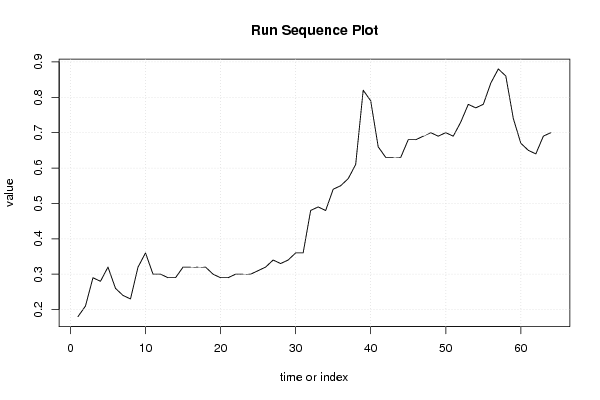
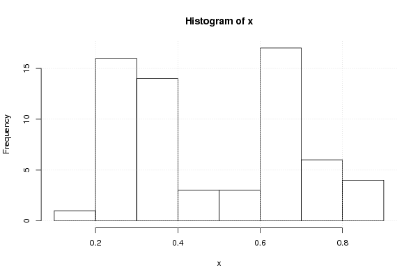
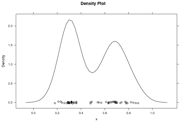
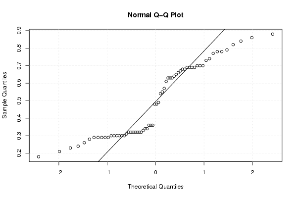
0,18
0,21
0,29
0,28
0,32
0,26
0,24
0,23
0,32
0,36
0,3
0,3
0,29
0,29
0,32
0,32
0,32
0,32
0,3
0,29
0,29
0,3
0,3
0,3
0,31
0,32
0,34
0,33
0,34
0,36
0,36
0,48
0,49
0,48
0,54
0,55
0,57
0,61
0,82
0,79
0,66
0,63
0,63
0,63
0,68
0,68
0,69
0,7
0,69
0,7
0,69
0,73
0,78
0,77
0,78
0,84
0,88
0,86
0,74
0,67
0,65
0,64
0,69
0,7

Summary of computational transaction
Raw Input	view raw input (R code)
Raw Output	view raw output of R engine
Computing time	2 seconds
R Server	'George Udny Yule' @ yule.wessa.net

\begin{tabular}{lllllllll}
\hline
Summary of computational transaction \tabularnewline
Raw Input & view raw input (R code)  \tabularnewline
Raw Output & view raw output of R engine  \tabularnewline
Computing time & 2 seconds \tabularnewline
R Server & 'George Udny Yule' @ yule.wessa.net \tabularnewline
\hline
\end{tabular}
%Source: https://freestatistics.org/blog/index.php?pk=145179&T=0

[TABLE]
[ROW][C]Summary of computational transaction[/C][/ROW]
[ROW][C]Raw Input[/C][C]view raw input (R code) [/C][/ROW]
[ROW][C]Raw Output[/C][C]view raw output of R engine [/C][/ROW]
[ROW][C]Computing time[/C][C]2 seconds[/C][/ROW]
[ROW][C]R Server[/C][C]'George Udny Yule' @ yule.wessa.net[/C][/ROW]
[/TABLE]
Source: https://freestatistics.org/blog/index.php?pk=145179&T=0

Globally Unique Identifier (entire table): ba.freestatistics.org/blog/index.php?pk=145179&T=0

As an alternative you can also use a QR Code:

The GUIDs for individual cells are displayed in the table below:

Summary of computational transaction
Raw Input	view raw input (R code)
Raw Output	view raw output of R engine
Computing time	2 seconds
R Server	'George Udny Yule' @ yule.wessa.net

Descriptive Statistics
# observations	64
minimum	0.18
Q1	0.3
median	0.48
mean	0.49578125
Q3	0.69
maximum	0.88

\begin{tabular}{lllllllll}
\hline
Descriptive Statistics \tabularnewline
# observations & 64 \tabularnewline
minimum & 0.18 \tabularnewline
Q1 & 0.3 \tabularnewline
median & 0.48 \tabularnewline
mean & 0.49578125 \tabularnewline
Q3 & 0.69 \tabularnewline
maximum & 0.88 \tabularnewline
\hline
\end{tabular}
%Source: https://freestatistics.org/blog/index.php?pk=145179&T=1

[TABLE]
[ROW][C]Descriptive Statistics[/C][/ROW]
[ROW][C]# observations[/C][C]64[/C][/ROW]
[ROW][C]minimum[/C][C]0.18[/C][/ROW]
[ROW][C]Q1[/C][C]0.3[/C][/ROW]
[ROW][C]median[/C][C]0.48[/C][/ROW]
[ROW][C]mean[/C][C]0.49578125[/C][/ROW]
[ROW][C]Q3[/C][C]0.69[/C][/ROW]
[ROW][C]maximum[/C][C]0.88[/C][/ROW]
[/TABLE]
Source: https://freestatistics.org/blog/index.php?pk=145179&T=1

Globally Unique Identifier (entire table): ba.freestatistics.org/blog/index.php?pk=145179&T=1

As an alternative you can also use a QR Code:

The GUIDs for individual cells are displayed in the table below:

Descriptive Statistics
# observations	64
minimum	0.18
Q1	0.3
median	0.48
mean	0.49578125
Q3	0.69
maximum	0.88

Figure 1

PNG link

Postscript link

PDF link

Figure 2

PNG link

Postscript link

PDF link

Figure 3

PNG link

Postscript link

PDF link

Figure 4

PNG link

Postscript link

PDF link

Figure 5

PNG link

Postscript link

PDF link

Figure 6

PNG link

Postscript link

PDF link

Figure 7

PNG link

Postscript link

PDF link

Parameters (Session):

par1 = 0 ; par2 = 0 ;

Parameters (R input):

par1 = 0 ; par2 = 0 ;

R code (references can be found in the software module):

par1 <- as.numeric(par1)
par2 <- as.numeric(par2)
x <- as.ts(x)
library(lattice)
bitmap(file='pic1.png')
plot(x,type='l',main='Run Sequence Plot',xlab='time or index',ylab='value')
grid()
dev.off()
bitmap(file='pic2.png')
hist(x)
grid()
dev.off()
bitmap(file='pic3.png')
if (par1 > 0)
{
densityplot(~x,col='black',main=paste('Density Plot   bw = ',par1),bw=par1)
} else {
densityplot(~x,col='black',main='Density Plot')
}
dev.off()
bitmap(file='pic4.png')
qqnorm(x)
qqline(x)
grid()
dev.off()
if (par2 > 0)
{
bitmap(file='lagplot1.png')
dum <- cbind(lag(x,k=1),x)
dum
dum1 <- dum[2:length(x),]
dum1
z <- as.data.frame(dum1)
z
plot(z,main='Lag plot (k=1), lowess, and regression line')
lines(lowess(z))
abline(lm(z))
dev.off()
if (par2 > 1) {
bitmap(file='lagplotpar2.png')
dum <- cbind(lag(x,k=par2),x)
dum
dum1 <- dum[(par2+1):length(x),]
dum1
z <- as.data.frame(dum1)
z
mylagtitle <- 'Lag plot (k='
mylagtitle <- paste(mylagtitle,par2,sep='')
mylagtitle <- paste(mylagtitle,'), and lowess',sep='')
plot(z,main=mylagtitle)
lines(lowess(z))
dev.off()
}
bitmap(file='pic5.png')
acf(x,lag.max=par2,main='Autocorrelation Function')
grid()
dev.off()
}
summary(x)
load(file='createtable')
a<-table.start()
a<-table.row.start(a)
a<-table.element(a,'Descriptive Statistics',2,TRUE)
a<-table.row.end(a)
a<-table.row.start(a)
a<-table.element(a,'# observations',header=TRUE)
a<-table.element(a,length(x))
a<-table.row.end(a)
a<-table.row.start(a)
a<-table.element(a,'minimum',header=TRUE)
a<-table.element(a,min(x))
a<-table.row.end(a)
a<-table.row.start(a)
a<-table.element(a,'Q1',header=TRUE)
a<-table.element(a,quantile(x,0.25))
a<-table.row.end(a)
a<-table.row.start(a)
a<-table.element(a,'median',header=TRUE)
a<-table.element(a,median(x))
a<-table.row.end(a)
a<-table.row.start(a)
a<-table.element(a,'mean',header=TRUE)
a<-table.element(a,mean(x))
a<-table.row.end(a)
a<-table.row.start(a)
a<-table.element(a,'Q3',header=TRUE)
a<-table.element(a,quantile(x,0.75))
a<-table.row.end(a)
a<-table.row.start(a)
a<-table.element(a,'maximum',header=TRUE)
a<-table.element(a,max(x))
a<-table.row.end(a)
a<-table.end(a)
table.save(a,file='mytable.tab')

Free Statistics

Description of Statistical Computation

Tree of Dependent Computations

Dataset

Tables (Output of Computation)

Figures (Output of Computation)

Input Parameters & R Code