Repository of Reproducible Computations

Free Statistics

of Irreproducible Research!

Author's title

Author

*The author of this computation has been verified*

R Software Module

rwasp_edauni.wasp

Title produced by software

Univariate Explorative Data Analysis

Date of computation

Thu, 17 Nov 2011 11:35:18 -0500

Cite this page as follows

Statistical Computations at FreeStatistics.org, Office for Research Development and Education, URL https://freestatistics.org/blog/index.php?v=date/2011/Nov/17/t13215477566e93fsj3ehie9dy.htm/, Retrieved Wed, 24 Apr 2024 22:32:39 +0000

Statistical Computations at FreeStatistics.org, Office for Research Development and Education, URL https://freestatistics.org/blog/index.php?pk=145086, Retrieved Wed, 24 Apr 2024 22:32:39 +0000

QR Codes:

Paste this QR Code to cite your computation.

Original text written by user:

IsPrivate?

No (this computation is public)

User-defined keywords

Estimated Impact

Family? (F = Feedback message, R = changed R code, M = changed R Module, P = changed Parameters, D = changed Data)

-     [Notched Boxplots] [3/11/2009] [2009-11-02 21:10:41] [b98453cac15ba1066b407e146608df68]
- R  D  [Notched Boxplots] [] [2009-12-18 14:47:51] [69c775ce4d55db2aa75a88e773e8d700]
- RMPD    [Univariate Data Series] [] [2009-12-21 16:28:58] [4409a44d89cea4fe559b38f99bc8a66c]
- R PD      [Univariate Data Series] [uni data] [2011-11-17 16:19:51] [141ef847e2c5f8e947fe4eabcb0cf143]
- RM D          [Univariate Explorative Data Analysis] [uni Eda] [2011-11-17 16:35:18] [1a4698f17d8e7f554418314cf0e4bd67] [Current]

Feedback Forum

Post a new message

Dataseries X:

Download CSV

Histogram

Boxplots

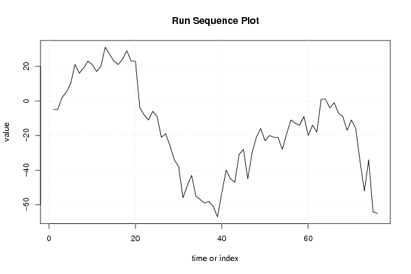
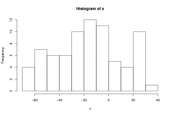
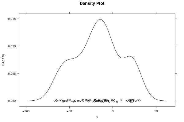
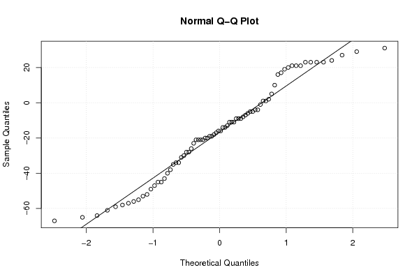
-5
-5
2
5
10
21
16
19
23
21
17
20
31
27
23
21
24
29
23
23
-4
-8
-11
-6
-9
-21
-19
-26
-34
-38
-56
-49
-43
-55
-57
-59
-58
-61
-67
-53
-40
-45
-47
-31
-28
-45
-30
-21
-16
-23
-20
-21
-21
-28
-19
-11
-13
-14
-9
-20
-14
-18
1
1
-4
-1
-7
-9
-17
-11
-16
-35
-52
-34
-64
-65

Summary of computational transaction
Raw Input	view raw input (R code)
Raw Output	view raw output of R engine
Computing time	2 seconds
R Server	'AstonUniversity' @ aston.wessa.net

\begin{tabular}{lllllllll}
\hline
Summary of computational transaction \tabularnewline
Raw Input & view raw input (R code)  \tabularnewline
Raw Output & view raw output of R engine  \tabularnewline
Computing time & 2 seconds \tabularnewline
R Server & 'AstonUniversity' @ aston.wessa.net \tabularnewline
\hline
\end{tabular}
%Source: https://freestatistics.org/blog/index.php?pk=145086&T=0

[TABLE]
[ROW][C]Summary of computational transaction[/C][/ROW]
[ROW][C]Raw Input[/C][C]view raw input (R code) [/C][/ROW]
[ROW][C]Raw Output[/C][C]view raw output of R engine [/C][/ROW]
[ROW][C]Computing time[/C][C]2 seconds[/C][/ROW]
[ROW][C]R Server[/C][C]'AstonUniversity' @ aston.wessa.net[/C][/ROW]
[/TABLE]
Source: https://freestatistics.org/blog/index.php?pk=145086&T=0

Globally Unique Identifier (entire table): ba.freestatistics.org/blog/index.php?pk=145086&T=0

As an alternative you can also use a QR Code:

The GUIDs for individual cells are displayed in the table below:

Summary of computational transaction
Raw Input	view raw input (R code)
Raw Output	view raw output of R engine
Computing time	2 seconds
R Server	'AstonUniversity' @ aston.wessa.net

Descriptive Statistics
# observations	76
minimum	-67
Q1	-34.25
median	-16
mean	-16.2631578947368
Q3	1
maximum	31

\begin{tabular}{lllllllll}
\hline
Descriptive Statistics \tabularnewline
# observations & 76 \tabularnewline
minimum & -67 \tabularnewline
Q1 & -34.25 \tabularnewline
median & -16 \tabularnewline
mean & -16.2631578947368 \tabularnewline
Q3 & 1 \tabularnewline
maximum & 31 \tabularnewline
\hline
\end{tabular}
%Source: https://freestatistics.org/blog/index.php?pk=145086&T=1

[TABLE]
[ROW][C]Descriptive Statistics[/C][/ROW]
[ROW][C]# observations[/C][C]76[/C][/ROW]
[ROW][C]minimum[/C][C]-67[/C][/ROW]
[ROW][C]Q1[/C][C]-34.25[/C][/ROW]
[ROW][C]median[/C][C]-16[/C][/ROW]
[ROW][C]mean[/C][C]-16.2631578947368[/C][/ROW]
[ROW][C]Q3[/C][C]1[/C][/ROW]
[ROW][C]maximum[/C][C]31[/C][/ROW]
[/TABLE]
Source: https://freestatistics.org/blog/index.php?pk=145086&T=1

Globally Unique Identifier (entire table): ba.freestatistics.org/blog/index.php?pk=145086&T=1

As an alternative you can also use a QR Code:

The GUIDs for individual cells are displayed in the table below:

Descriptive Statistics
# observations	76
minimum	-67
Q1	-34.25
median	-16
mean	-16.2631578947368
Q3	1
maximum	31

Figure 1

PNG link

Postscript link

PDF link

Figure 2

PNG link

Postscript link

PDF link

Figure 3

PNG link

Postscript link

PDF link

Figure 4

PNG link

Postscript link

PDF link

Figure 5

PNG link

Postscript link

PDF link

Figure 6

PNG link

Postscript link

PDF link

Figure 7

PNG link

Postscript link

PDF link

Parameters (Session):

par1 = 12 ;

Parameters (R input):

par1 = 0 ; par2 = 0 ;

R code (references can be found in the software module):

par1 <- as.numeric(par1)
par2 <- as.numeric(par2)
x <- as.ts(x)
library(lattice)
bitmap(file='pic1.png')
plot(x,type='l',main='Run Sequence Plot',xlab='time or index',ylab='value')
grid()
dev.off()
bitmap(file='pic2.png')
hist(x)
grid()
dev.off()
bitmap(file='pic3.png')
if (par1 > 0)
{
densityplot(~x,col='black',main=paste('Density Plot   bw = ',par1),bw=par1)
} else {
densityplot(~x,col='black',main='Density Plot')
}
dev.off()
bitmap(file='pic4.png')
qqnorm(x)
qqline(x)
grid()
dev.off()
if (par2 > 0)
{
bitmap(file='lagplot1.png')
dum <- cbind(lag(x,k=1),x)
dum
dum1 <- dum[2:length(x),]
dum1
z <- as.data.frame(dum1)
z
plot(z,main='Lag plot (k=1), lowess, and regression line')
lines(lowess(z))
abline(lm(z))
dev.off()
if (par2 > 1) {
bitmap(file='lagplotpar2.png')
dum <- cbind(lag(x,k=par2),x)
dum
dum1 <- dum[(par2+1):length(x),]
dum1
z <- as.data.frame(dum1)
z
mylagtitle <- 'Lag plot (k='
mylagtitle <- paste(mylagtitle,par2,sep='')
mylagtitle <- paste(mylagtitle,'), and lowess',sep='')
plot(z,main=mylagtitle)
lines(lowess(z))
dev.off()
}
bitmap(file='pic5.png')
acf(x,lag.max=par2,main='Autocorrelation Function')
grid()
dev.off()
}
summary(x)
load(file='createtable')
a<-table.start()
a<-table.row.start(a)
a<-table.element(a,'Descriptive Statistics',2,TRUE)
a<-table.row.end(a)
a<-table.row.start(a)
a<-table.element(a,'# observations',header=TRUE)
a<-table.element(a,length(x))
a<-table.row.end(a)
a<-table.row.start(a)
a<-table.element(a,'minimum',header=TRUE)
a<-table.element(a,min(x))
a<-table.row.end(a)
a<-table.row.start(a)
a<-table.element(a,'Q1',header=TRUE)
a<-table.element(a,quantile(x,0.25))
a<-table.row.end(a)
a<-table.row.start(a)
a<-table.element(a,'median',header=TRUE)
a<-table.element(a,median(x))
a<-table.row.end(a)
a<-table.row.start(a)
a<-table.element(a,'mean',header=TRUE)
a<-table.element(a,mean(x))
a<-table.row.end(a)
a<-table.row.start(a)
a<-table.element(a,'Q3',header=TRUE)
a<-table.element(a,quantile(x,0.75))
a<-table.row.end(a)
a<-table.row.start(a)
a<-table.element(a,'maximum',header=TRUE)
a<-table.element(a,max(x))
a<-table.row.end(a)
a<-table.end(a)
table.save(a,file='mytable.tab')

Free Statistics

Description of Statistical Computation

Tree of Dependent Computations

Dataset

Tables (Output of Computation)

Figures (Output of Computation)

Input Parameters & R Code