Free Statistics
of Irreproducible Research!
Description of Statistical Computation | |||||||||||||||||||||
|---|---|---|---|---|---|---|---|---|---|---|---|---|---|---|---|---|---|---|---|---|---|
| Author's title | |||||||||||||||||||||
| Author | *The author of this computation has been verified* | ||||||||||||||||||||
| R Software Module | rwasp_meanplot.wasp | ||||||||||||||||||||
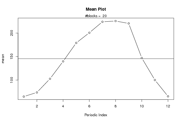
| Title produced by software | Mean Plot | ||||||||||||||||||||
| Date of computation | Thu, 17 Nov 2011 11:11:46 -0500 | ||||||||||||||||||||
| Cite this page as follows | Statistical Computations at FreeStatistics.org, Office for Research Development and Education, URL https://freestatistics.org/blog/index.php?v=date/2011/Nov/17/t1321546326wpf74xx7unrqu7s.htm/, Retrieved Sat, 20 Apr 2024 02:23:14 +0000 | ||||||||||||||||||||
| Statistical Computations at FreeStatistics.org, Office for Research Development and Education, URL https://freestatistics.org/blog/index.php?pk=145031, Retrieved Sat, 20 Apr 2024 02:23:14 +0000 | |||||||||||||||||||||
| QR Codes: | |||||||||||||||||||||
|
| |||||||||||||||||||||
| Original text written by user: | |||||||||||||||||||||
| IsPrivate? | No (this computation is public) | ||||||||||||||||||||
| User-defined keywords | |||||||||||||||||||||
| Estimated Impact | 58 | ||||||||||||||||||||
Tree of Dependent Computations | |||||||||||||||||||||
| Family? (F = Feedback message, R = changed R code, M = changed R Module, P = changed Parameters, D = changed Data) | |||||||||||||||||||||
| - [Bivariate Data Series] [Bivariate dataset] [2008-01-05 23:51:08] [74be16979710d4c4e7c6647856088456] - RMPD [Blocked Bootstrap Plot - Central Tendency] [Colombia Coffee] [2008-01-07 10:26:26] [74be16979710d4c4e7c6647856088456] - RMPD [Mean Plot] [Mean Plot Yt] [2011-11-17 16:11:46] [e5e604418bec6ffe5109fb01f8a59ccb] [Current] | |||||||||||||||||||||
| Feedback Forum | |||||||||||||||||||||
Post a new message | |||||||||||||||||||||
Dataset | |||||||||||||||||||||
| Dataseries X: | |||||||||||||||||||||
80 111 122 131 192 188 216 238 173 160 93 67 60 32 126 131 134 162 230 232 200 143 85 66 54 81 100 126 204 218 227 220 220 120 110 67 81 52 106 156 187 204 204 196 204 124 53 77 77 50 105 125 165 194 263 225 263 140 127 86 71 95 95 133 178 160 250 251 250 173 103 21 29 39 71 148 144 199 206 224 206 152 88 35 23 92 117 120 173 202 217 256 217 143 95 77 76 100 108 132 195 198 204 212 204 129 73 77 80 64 109 138 185 198 237 223 237 146 102 77 70 86 98 141 195 205 191 226 191 147 100 74 56 77 80 120 186 196 229 229 229 176 104 61 72 99 113 140 174 209 205 229 215 136 113 57 55 66 125 149 176 230 238 245 238 124 111 72 63 78 100 149 166 201 214 231 214 151 97 68 81 55 99 146 170 218 218 207 218 178 105 67 47 55 73 124 185 213 278 205 278 171 125 92 96 92 118 185 183 215 207 214 207 142 102 66 87 90 90 133 205 201 220 210 220 136 95 52 40 60 100 169 184 202 226 239 226 149 121 50 | |||||||||||||||||||||
Tables (Output of Computation) | |||||||||||||||||||||
| |||||||||||||||||||||
Figures (Output of Computation) | |||||||||||||||||||||
Input Parameters & R Code | |||||||||||||||||||||
| Parameters (Session): | |||||||||||||||||||||
| par1 = 12 ; | |||||||||||||||||||||
| Parameters (R input): | |||||||||||||||||||||
| par1 = 12 ; | |||||||||||||||||||||
| R code (references can be found in the software module): | |||||||||||||||||||||
par1 <- as.numeric(par1) | |||||||||||||||||||||