Free Statistics
of Irreproducible Research!
Description of Statistical Computation | |||||||||||||||||||||||||||||||||||||||||||||||||||||||||||||
|---|---|---|---|---|---|---|---|---|---|---|---|---|---|---|---|---|---|---|---|---|---|---|---|---|---|---|---|---|---|---|---|---|---|---|---|---|---|---|---|---|---|---|---|---|---|---|---|---|---|---|---|---|---|---|---|---|---|---|---|---|---|
| Author's title | |||||||||||||||||||||||||||||||||||||||||||||||||||||||||||||
| Author | *The author of this computation has been verified* | ||||||||||||||||||||||||||||||||||||||||||||||||||||||||||||
| R Software Module | rwasp_linear_regression.wasp | ||||||||||||||||||||||||||||||||||||||||||||||||||||||||||||
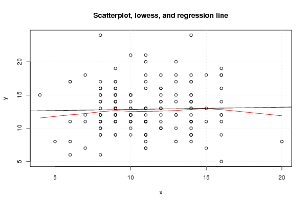
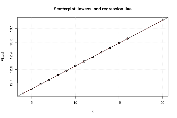
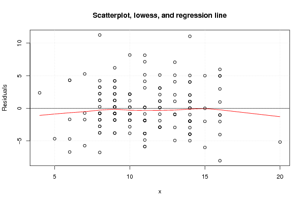
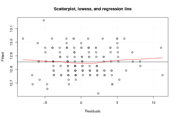
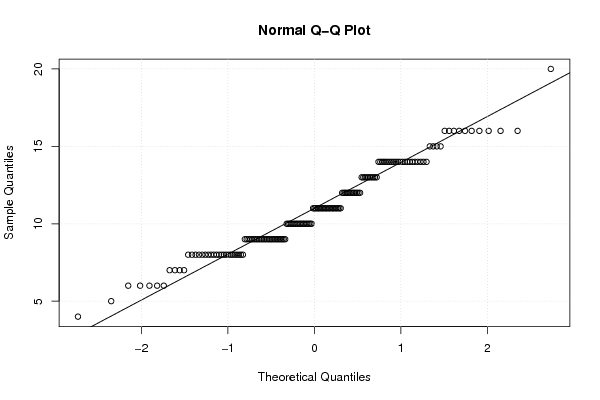
| Title produced by software | Linear Regression Graphical Model Validation | ||||||||||||||||||||||||||||||||||||||||||||||||||||||||||||
| Date of computation | Tue, 15 Nov 2011 18:39:00 -0500 | ||||||||||||||||||||||||||||||||||||||||||||||||||||||||||||
| Cite this page as follows | Statistical Computations at FreeStatistics.org, Office for Research Development and Education, URL https://freestatistics.org/blog/index.php?v=date/2011/Nov/15/t1321400360606y1bu9kvflw87.htm/, Retrieved Thu, 18 Apr 2024 11:00:25 +0000 | ||||||||||||||||||||||||||||||||||||||||||||||||||||||||||||
| Statistical Computations at FreeStatistics.org, Office for Research Development and Education, URL https://freestatistics.org/blog/index.php?pk=143686, Retrieved Thu, 18 Apr 2024 11:00:25 +0000 | |||||||||||||||||||||||||||||||||||||||||||||||||||||||||||||
| QR Codes: | |||||||||||||||||||||||||||||||||||||||||||||||||||||||||||||
|
| |||||||||||||||||||||||||||||||||||||||||||||||||||||||||||||
| Original text written by user: | |||||||||||||||||||||||||||||||||||||||||||||||||||||||||||||
| IsPrivate? | No (this computation is public) | ||||||||||||||||||||||||||||||||||||||||||||||||||||||||||||
| User-defined keywords | |||||||||||||||||||||||||||||||||||||||||||||||||||||||||||||
| Estimated Impact | 63 | ||||||||||||||||||||||||||||||||||||||||||||||||||||||||||||
Tree of Dependent Computations | |||||||||||||||||||||||||||||||||||||||||||||||||||||||||||||
| Family? (F = Feedback message, R = changed R code, M = changed R Module, P = changed Parameters, D = changed Data) | |||||||||||||||||||||||||||||||||||||||||||||||||||||||||||||
| - [Linear Regression Graphical Model Validation] [Colombia Coffee -...] [2008-02-26 10:22:06] [74be16979710d4c4e7c6647856088456] - M D [Linear Regression Graphical Model Validation] [Regression Model 1] [2010-11-16 09:46:35] [1429a1a14191a86916b95357f6de790b] - D [Linear Regression Graphical Model Validation] [Regression Model 2] [2010-11-16 17:18:05] [1429a1a14191a86916b95357f6de790b] - R P [Linear Regression Graphical Model Validation] [Workshop 6 - Mini...] [2011-11-15 23:39:00] [c18e83883fa784c15a15b4fbc0636edd] [Current] | |||||||||||||||||||||||||||||||||||||||||||||||||||||||||||||
| Feedback Forum | |||||||||||||||||||||||||||||||||||||||||||||||||||||||||||||
Post a new message | |||||||||||||||||||||||||||||||||||||||||||||||||||||||||||||
Dataset | |||||||||||||||||||||||||||||||||||||||||||||||||||||||||||||
| Dataseries X: | |||||||||||||||||||||||||||||||||||||||||||||||||||||||||||||
14 11 6 12 8 10 10 11 16 11 13 12 8 12 11 4 9 8 8 14 15 16 9 14 11 8 9 9 9 9 10 16 11 8 9 16 11 16 12 12 14 9 10 9 10 12 14 14 10 14 16 9 10 6 8 13 10 8 7 15 9 10 12 13 10 11 8 9 13 11 8 9 9 15 9 10 14 12 12 11 14 6 12 8 14 11 10 14 12 10 14 5 11 10 9 10 16 13 9 10 10 7 9 8 14 14 8 9 14 14 8 8 8 7 6 8 6 11 14 11 11 11 14 8 20 11 8 11 10 14 11 9 9 8 10 13 13 12 8 13 14 12 14 15 13 16 9 9 9 8 7 16 11 9 11 9 14 13 16 | |||||||||||||||||||||||||||||||||||||||||||||||||||||||||||||
| Dataseries Y: | |||||||||||||||||||||||||||||||||||||||||||||||||||||||||||||
11 7 17 10 12 12 11 11 12 13 14 16 11 10 11 15 9 11 17 17 11 18 14 10 11 15 15 13 16 13 9 18 18 12 17 9 9 12 18 12 18 14 15 16 10 11 14 9 12 17 5 12 12 6 24 12 12 14 7 13 12 13 14 8 11 9 11 13 10 11 12 9 15 18 15 12 13 14 10 13 13 11 13 16 8 16 11 9 16 12 14 8 9 15 11 21 14 18 12 13 15 12 19 15 11 11 10 13 15 12 12 16 9 18 8 13 17 9 15 8 7 12 14 6 8 17 10 11 14 11 13 12 11 9 12 20 12 13 12 12 9 15 24 7 17 11 17 11 12 14 11 16 21 14 20 13 11 15 19 | |||||||||||||||||||||||||||||||||||||||||||||||||||||||||||||
Tables (Output of Computation) | |||||||||||||||||||||||||||||||||||||||||||||||||||||||||||||
| |||||||||||||||||||||||||||||||||||||||||||||||||||||||||||||
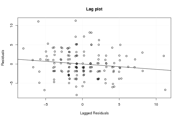
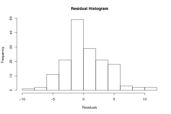
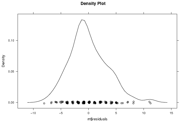
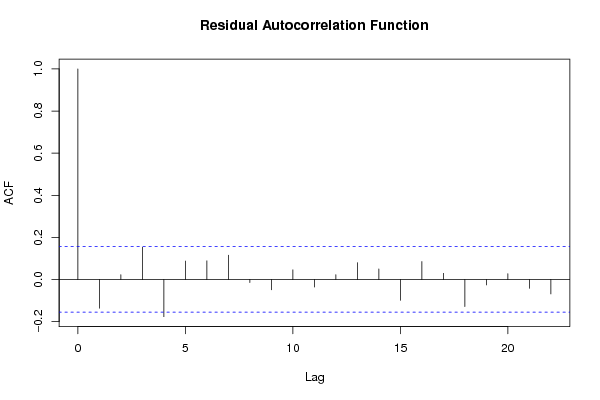
Figures (Output of Computation) | |||||||||||||||||||||||||||||||||||||||||||||||||||||||||||||
Input Parameters & R Code | |||||||||||||||||||||||||||||||||||||||||||||||||||||||||||||
| Parameters (Session): | |||||||||||||||||||||||||||||||||||||||||||||||||||||||||||||
| par1 = 1 ; par2 = 4 ; par3 = Pearson Chi-Squared ; | |||||||||||||||||||||||||||||||||||||||||||||||||||||||||||||
| Parameters (R input): | |||||||||||||||||||||||||||||||||||||||||||||||||||||||||||||
| par1 = 0 ; | |||||||||||||||||||||||||||||||||||||||||||||||||||||||||||||
| R code (references can be found in the software module): | |||||||||||||||||||||||||||||||||||||||||||||||||||||||||||||
par1 <- as.numeric(par1) | |||||||||||||||||||||||||||||||||||||||||||||||||||||||||||||