Free Statistics
of Irreproducible Research!
Description of Statistical Computation | |||||||||||||||||||||||||||||||||||||||||||||||||||||||||||||
|---|---|---|---|---|---|---|---|---|---|---|---|---|---|---|---|---|---|---|---|---|---|---|---|---|---|---|---|---|---|---|---|---|---|---|---|---|---|---|---|---|---|---|---|---|---|---|---|---|---|---|---|---|---|---|---|---|---|---|---|---|---|
| Author's title | |||||||||||||||||||||||||||||||||||||||||||||||||||||||||||||
| Author | *The author of this computation has been verified* | ||||||||||||||||||||||||||||||||||||||||||||||||||||||||||||
| R Software Module | -- | ||||||||||||||||||||||||||||||||||||||||||||||||||||||||||||
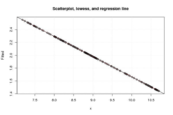
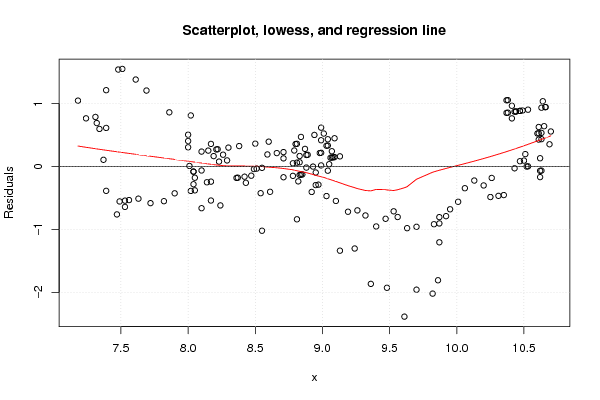
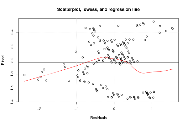
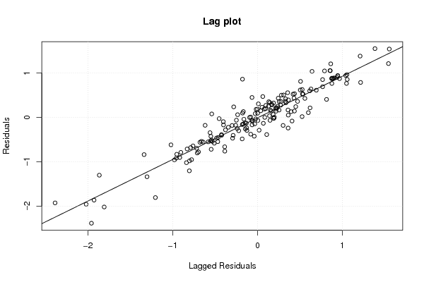
| Title produced by software | Linear Regression Graphical Model Validation | ||||||||||||||||||||||||||||||||||||||||||||||||||||||||||||
| Date of computation | Tue, 15 Nov 2011 17:53:52 -0500 | ||||||||||||||||||||||||||||||||||||||||||||||||||||||||||||
| Cite this page as follows | Statistical Computations at FreeStatistics.org, Office for Research Development and Education, URL https://freestatistics.org/blog/index.php?v=date/2011/Nov/15/t1321397641g6teia0mahkuhxv.htm/, Retrieved Sat, 27 Apr 2024 01:42:44 +0000 | ||||||||||||||||||||||||||||||||||||||||||||||||||||||||||||
| Statistical Computations at FreeStatistics.org, Office for Research Development and Education, URL https://freestatistics.org/blog/index.php?pk=143653, Retrieved Sat, 27 Apr 2024 01:42:44 +0000 | |||||||||||||||||||||||||||||||||||||||||||||||||||||||||||||
| QR Codes: | |||||||||||||||||||||||||||||||||||||||||||||||||||||||||||||
|
| |||||||||||||||||||||||||||||||||||||||||||||||||||||||||||||
| Original text written by user: | |||||||||||||||||||||||||||||||||||||||||||||||||||||||||||||
| IsPrivate? | No (this computation is public) | ||||||||||||||||||||||||||||||||||||||||||||||||||||||||||||
| User-defined keywords | |||||||||||||||||||||||||||||||||||||||||||||||||||||||||||||
| Estimated Impact | 136 | ||||||||||||||||||||||||||||||||||||||||||||||||||||||||||||
Tree of Dependent Computations | |||||||||||||||||||||||||||||||||||||||||||||||||||||||||||||
| Family? (F = Feedback message, R = changed R code, M = changed R Module, P = changed Parameters, D = changed Data) | |||||||||||||||||||||||||||||||||||||||||||||||||||||||||||||
| - [Linear Regression Graphical Model Validation] [Colombia Coffee -...] [2008-02-26 10:22:06] [74be16979710d4c4e7c6647856088456] - RM D [Linear Regression Graphical Model Validation] [WS6 - Mini Tutori...] [2010-11-12 08:44:11] [1f5baf2b24e732d76900bb8178fc04e7] - RM [Linear Regression Graphical Model Validation] [] [2011-11-15 22:53:52] [0f9b7c3b8d01420b2751adc6f98a35df] [Current] | |||||||||||||||||||||||||||||||||||||||||||||||||||||||||||||
| Feedback Forum | |||||||||||||||||||||||||||||||||||||||||||||||||||||||||||||
Post a new message | |||||||||||||||||||||||||||||||||||||||||||||||||||||||||||||
Dataset | |||||||||||||||||||||||||||||||||||||||||||||||||||||||||||||
| Dataseries X: | |||||||||||||||||||||||||||||||||||||||||||||||||||||||||||||
10,47 10,44 10,41 10,37 10,38 10,38 10,37 10,41 10,44 10,43 10,47 10,49 10,53 10,63 10,66 10,66 10,64 10,65 10,61 10,6 10,61 10,63 10,63 10,61 10,7 10,69 10,62 10,62 10,63 10,62 10,53 10,51 10,5 10,52 10,47 10,43 10,35 10,31 10,25 10,26 10,2 10,13 10,06 10,01 9,95 9,92 9,87 9,83 9,7 9,63 9,56 9,53 9,47 9,4 9,32 9,26 9,19 9,1 9,03 8,95 8,85 8,78 8,71 8,61 8,54 8,49 8,42 8,36 8,3 8,19 8,15 8,1 8,04 8,05 8,04 8 8,02 8 8 8,01 8,04 8,1 8,14 8,17 8,17 8,22 8,21 8,29 8,37 8,43 8,47 8,51 8,55 8,59 8,66 8,71 8,78 8,81 8,84 8,81 8,82 8,84 8,83 8,83 8,88 8,88 8,89 8,93 8,95 8,92 8,97 8,99 9,01 8,99 9,03 9,04 9,07 9,04 9,07 9,09 9,04 9,08 9,13 9,09 9,05 9,06 8,99 8,98 8,99 8,94 8,87 8,83 8,8 8,79 8,71 8,6 8,5 8,38 8,26 8,23 8,17 8,1 8,02 7,9 7,82 7,72 7,63 7,53 7,56 7,49 7,53 7,47 7,39 7,37 7,34 7,39 7,32 7,24 7,18 7,31 7,39 7,48 7,51 7,61 7,69 7,86 8,05 8,24 8,55 8,81 9,13 9,24 9,36 9,48 9,61 9,7 9,82 9,86 9,87 9,87 | |||||||||||||||||||||||||||||||||||||||||||||||||||||||||||||
| Dataseries Y: | |||||||||||||||||||||||||||||||||||||||||||||||||||||||||||||
2,4 2,4 2,5 2,6 2,4 2,6 2,4 2,3 2,4 2,4 2,4 2,4 2,4 2,4 2,4 2,4 2,5 2,1 2,1 2 2 2 1,9 1,9 2 1,8 1,6 1,3 1,4 1,4 1,5 1,7 1,6 1,5 1,6 1,5 1,1 1,1 1,1 1,4 1,3 1,4 1,3 1,1 1 0,9 0,8 0,8 0,8 0,8 1 1,1 1 0,9 1,1 1,2 1,2 1,4 1,5 1,7 1,9 1,9 1,9 1,7 1,7 2,1 2 2 2,5 2,4 2,5 2,5 2 1,9 2,2 2,7 3,1 2,8 2,6 2,3 2,2 2,2 2 2 2,6 2,5 2,5 2,3 2 1,9 2 2,1 2,1 2,3 2,3 2,3 2,1 2,4 2,5 2,1 1,8 1,9 1,9 2,1 2,2 2 2,2 2 1,9 1,6 1,7 2 2,5 2,4 2,3 2,3 2,1 2,4 2,2 2,4 1,9 2,1 2,1 2,1 2 2,1 2,2 2,2 2,6 2,5 2,3 2,2 2,4 2,3 2,2 2,5 2,5 2,5 2,4 2,3 1,7 1,6 1,9 1,9 1,8 1,8 1,9 1,9 1,9 1,9 1,8 1,7 2,1 2,6 3,1 3,1 3,2 3,3 3,6 3,3 3,7 4 4 3,8 3,6 3,2 2,1 1,6 1,1 1,2 0,6 0,6 0 -0,1 -0,6 -0,2 -0,3 -0,1 0,5 0,9 | |||||||||||||||||||||||||||||||||||||||||||||||||||||||||||||
Tables (Output of Computation) | |||||||||||||||||||||||||||||||||||||||||||||||||||||||||||||
| |||||||||||||||||||||||||||||||||||||||||||||||||||||||||||||
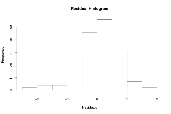
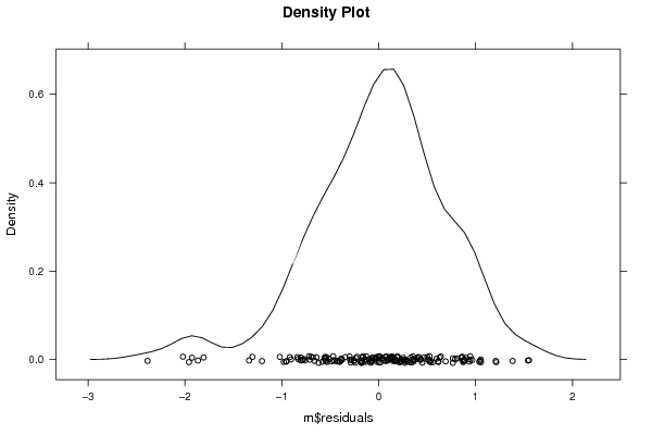
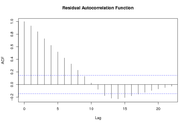
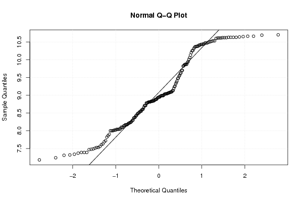
Figures (Output of Computation) | |||||||||||||||||||||||||||||||||||||||||||||||||||||||||||||
Input Parameters & R Code | |||||||||||||||||||||||||||||||||||||||||||||||||||||||||||||
| Parameters (Session): | |||||||||||||||||||||||||||||||||||||||||||||||||||||||||||||
| par1 = 0 ; | |||||||||||||||||||||||||||||||||||||||||||||||||||||||||||||
| Parameters (R input): | |||||||||||||||||||||||||||||||||||||||||||||||||||||||||||||
| par1 = 0 ; par2 = ; par3 = ; par4 = ; par5 = ; par6 = ; par7 = ; par8 = ; par9 = ; par10 = ; par11 = ; par12 = ; par13 = ; par14 = ; par15 = ; par16 = ; par17 = ; par18 = ; par19 = ; par20 = ; | |||||||||||||||||||||||||||||||||||||||||||||||||||||||||||||
| R code (references can be found in the software module): | |||||||||||||||||||||||||||||||||||||||||||||||||||||||||||||
par1 <- as.numeric(par1) | |||||||||||||||||||||||||||||||||||||||||||||||||||||||||||||