Free Statistics
of Irreproducible Research!
Description of Statistical Computation | |||||||||||||||||||||||||||||||||||||||||||||||||||||||||||||
|---|---|---|---|---|---|---|---|---|---|---|---|---|---|---|---|---|---|---|---|---|---|---|---|---|---|---|---|---|---|---|---|---|---|---|---|---|---|---|---|---|---|---|---|---|---|---|---|---|---|---|---|---|---|---|---|---|---|---|---|---|---|
| Author's title | |||||||||||||||||||||||||||||||||||||||||||||||||||||||||||||
| Author | *Unverified author* | ||||||||||||||||||||||||||||||||||||||||||||||||||||||||||||
| R Software Module | rwasp_linear_regression.wasp | ||||||||||||||||||||||||||||||||||||||||||||||||||||||||||||
| Title produced by software | Linear Regression Graphical Model Validation | ||||||||||||||||||||||||||||||||||||||||||||||||||||||||||||
| Date of computation | Tue, 15 Nov 2011 17:38:28 -0500 | ||||||||||||||||||||||||||||||||||||||||||||||||||||||||||||
| Cite this page as follows | Statistical Computations at FreeStatistics.org, Office for Research Development and Education, URL https://freestatistics.org/blog/index.php?v=date/2011/Nov/15/t1321396778c6yvj8n1e1f801d.htm/, Retrieved Fri, 19 Apr 2024 05:52:31 +0000 | ||||||||||||||||||||||||||||||||||||||||||||||||||||||||||||
| Statistical Computations at FreeStatistics.org, Office for Research Development and Education, URL https://freestatistics.org/blog/index.php?pk=143634, Retrieved Fri, 19 Apr 2024 05:52:31 +0000 | |||||||||||||||||||||||||||||||||||||||||||||||||||||||||||||
| QR Codes: | |||||||||||||||||||||||||||||||||||||||||||||||||||||||||||||
|
| |||||||||||||||||||||||||||||||||||||||||||||||||||||||||||||
| Original text written by user: | |||||||||||||||||||||||||||||||||||||||||||||||||||||||||||||
| IsPrivate? | No (this computation is public) | ||||||||||||||||||||||||||||||||||||||||||||||||||||||||||||
| User-defined keywords | |||||||||||||||||||||||||||||||||||||||||||||||||||||||||||||
| Estimated Impact | 76 | ||||||||||||||||||||||||||||||||||||||||||||||||||||||||||||
Tree of Dependent Computations | |||||||||||||||||||||||||||||||||||||||||||||||||||||||||||||
| Family? (F = Feedback message, R = changed R code, M = changed R Module, P = changed Parameters, D = changed Data) | |||||||||||||||||||||||||||||||||||||||||||||||||||||||||||||
| - [Linear Regression Graphical Model Validation] [Colombia Coffee -...] [2008-02-26 10:22:06] [74be16979710d4c4e7c6647856088456] - RM D [Linear Regression Graphical Model Validation] [Tutorial] [2011-11-15 22:38:28] [d41d8cd98f00b204e9800998ecf8427e] [Current] - D [Linear Regression Graphical Model Validation] [ws6 tutorial] [2011-11-15 22:50:40] [74be16979710d4c4e7c6647856088456] | |||||||||||||||||||||||||||||||||||||||||||||||||||||||||||||
| Feedback Forum | |||||||||||||||||||||||||||||||||||||||||||||||||||||||||||||
Post a new message | |||||||||||||||||||||||||||||||||||||||||||||||||||||||||||||
Dataset | |||||||||||||||||||||||||||||||||||||||||||||||||||||||||||||
| Dataseries X: | |||||||||||||||||||||||||||||||||||||||||||||||||||||||||||||
93,09 94,84 93,53 95,5 94,52 95,33 97,45 98,2 97,7 98,68 97,43 97,8 98,1 96,86 97,72 96,63 95,27 97,66 97,72 99,42 101,59 101,93 102,01 103,13 102,2 99,08 100,52 102,01 101,7 101 103,06 101,45 103,24 102,24 102,71 105,74 106,06 110,89 112,06 111,78 111,88 114,88 116,65 114,53 115,89 115,53 113,3 115,7 115,79 113,71 113,67 108,52 111,05 114,9 113,93 114,96 114,96 115,7 115,72 115,59 115,1 115,27 115,17 115,17 115,27 115,17 115,27 115,17 122,3 122,67 126,65 123,98 122,88 122,36 123,45 121,61 121,33 123,85 123,99 124,04 123,66 124,14 125,13 125,02 125,89 125,12 122,45 121,19 110,8 109,13 115,9 117,63 112,57 112,98 113,83 112,73 109,99 112,3 111,42 112,39 110,1 112,53 114,93 115,05 115,03 114,68 116,63 114,53 115,54 115,84 114,48 116,78 117,85 119,57 118,78 119,1 120,16 113,01 114,02 113,21 111,69 112,1 114,21 107,26 105,12 105,99 108,78 112,4 112,48 117,77 111,39 113,61 113,62 118,59 118,33 117,03 117,75 118,78 118,32 117,26 116,05 117,06 118,15 117,51 118,67 117,94 118,28 117,43 117,36 116,74 116,81 116,46 113,23 107,25 109,37 103,74 102,57 106,68 108,02 108,03 109,91 109,47 110,6 106,99 108,62 108,11 108,36 109,31 110,69 111,36 111,88 114,02 114,85 114,29 112,33 110,08 112,89 115,69 114,55 112,77 112,25 111,89 112,4 115,34 112,22 109,14 110,54 110,36 105,49 103,97 103,94 107,14 103,81 103,95 102,76 101,71 99,79 102,73 105,73 105,88 108,95 111,12 111,36 111,11 114,68 110,16 111,15 108,39 109,76 109,56 109,56 111,45 108,91 112,08 109,91 109,56 | |||||||||||||||||||||||||||||||||||||||||||||||||||||||||||||
| Dataseries Y: | |||||||||||||||||||||||||||||||||||||||||||||||||||||||||||||
3035 2932 2852 2830 2850 2881 2934 2959 2952 3019 3019 3036 3100 3178 3184 3312 3335 3352 3358 3277 3352 3313 3352 3358 3251 3223 3239 3272 3397 3374 3400 3410 3463 3482 3546 3546 3633 3661 3684 3698 3757 3660 3701 3774 3697 3721 3703 3585 3490 3460 3431 3294 3233 3282 3127 3189 3263 3251 3203 3242 3248 3057 2987 2952 3011 3020 2975 2999 2987 2974 3022 3053 3066 3125 3239 3127 3117 3131 3130 3130 3128 3131 3206 3330 3390 3353 3271 3236 3087 3137 3143 3135 3115 3035 3000 3006 2980 2995 2979 2902 2865 2884 2962 3010 3010 2973 2999 2953 2904 2878 2863 2891 2927 2980 2997 3001 3014 2987 2914 2917 2967 3027 3040 2986 2967 2995 3018 3114 3170 3170 3142 3228 3202 3194 3099 3058 3076 3180 3166 3168 3186 3187 3207 3194 3093 3025 3047 3073 3011 3008 2989 2965 2952 2941 2975 2945 2943 2871 2871 2943 2871 2943 2871 2871 2943 2871 2943 2871 2871 2943 2871 2943 2871 3060 3067 3092 3067 3092 3092 3067 3092 3067 3092 3092 2792 2716 2730 2727 2680 2634 2678 2721 2664 2694 2608 2575 2592 2622 2660 2562 2684 2632 2659 2658 2700 2650 2610 2644 2607 2611 2670 2683 2727 2779 2770 2723 | |||||||||||||||||||||||||||||||||||||||||||||||||||||||||||||
Tables (Output of Computation) | |||||||||||||||||||||||||||||||||||||||||||||||||||||||||||||
| |||||||||||||||||||||||||||||||||||||||||||||||||||||||||||||
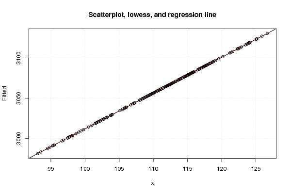
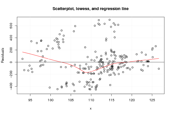
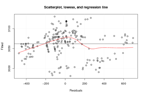
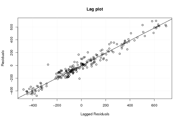
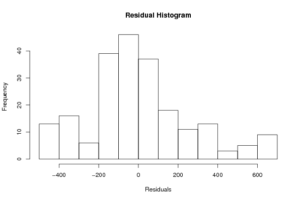
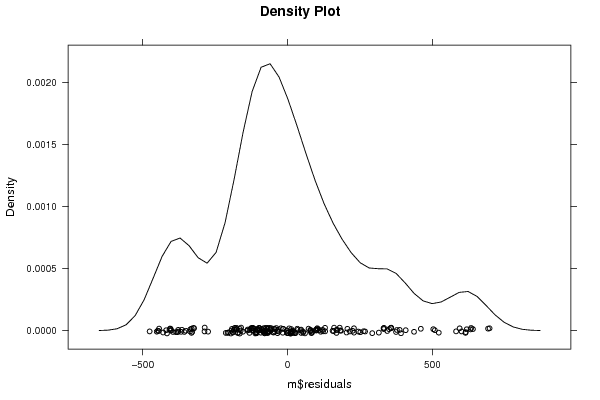
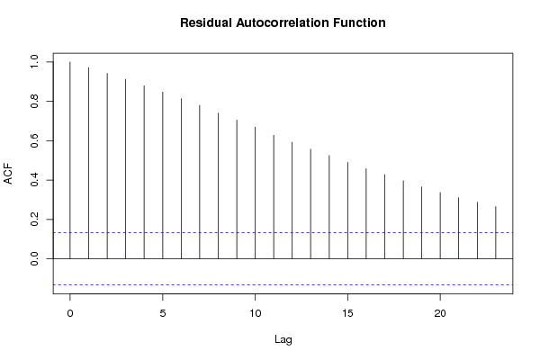
Figures (Output of Computation) | |||||||||||||||||||||||||||||||||||||||||||||||||||||||||||||
Input Parameters & R Code | |||||||||||||||||||||||||||||||||||||||||||||||||||||||||||||
| Parameters (Session): | |||||||||||||||||||||||||||||||||||||||||||||||||||||||||||||
| par1 = 0 ; | |||||||||||||||||||||||||||||||||||||||||||||||||||||||||||||
| Parameters (R input): | |||||||||||||||||||||||||||||||||||||||||||||||||||||||||||||
| par1 = 0 ; | |||||||||||||||||||||||||||||||||||||||||||||||||||||||||||||
| R code (references can be found in the software module): | |||||||||||||||||||||||||||||||||||||||||||||||||||||||||||||
par1 <- as.numeric(par1) | |||||||||||||||||||||||||||||||||||||||||||||||||||||||||||||