Free Statistics
of Irreproducible Research!
Description of Statistical Computation | |||||||||||||||||||||
|---|---|---|---|---|---|---|---|---|---|---|---|---|---|---|---|---|---|---|---|---|---|
| Author's title | |||||||||||||||||||||
| Author | *Unverified author* | ||||||||||||||||||||
| R Software Module | rwasp_meanplot.wasp | ||||||||||||||||||||
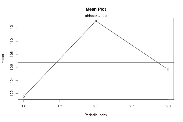
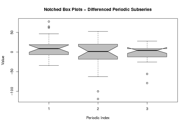
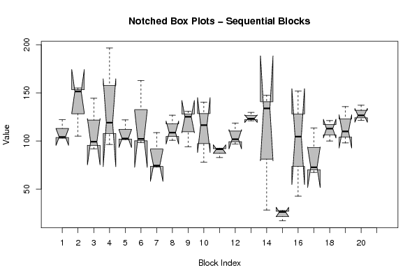
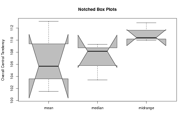
| Title produced by software | Mean Plot | ||||||||||||||||||||
| Date of computation | Tue, 15 Nov 2011 15:28:55 -0500 | ||||||||||||||||||||
| Cite this page as follows | Statistical Computations at FreeStatistics.org, Office for Research Development and Education, URL https://freestatistics.org/blog/index.php?v=date/2011/Nov/15/t1321388973p5zuavj0sel2qnd.htm/, Retrieved Fri, 26 Apr 2024 04:26:09 +0000 | ||||||||||||||||||||
| Statistical Computations at FreeStatistics.org, Office for Research Development and Education, URL https://freestatistics.org/blog/index.php?pk=143503, Retrieved Fri, 26 Apr 2024 04:26:09 +0000 | |||||||||||||||||||||
| QR Codes: | |||||||||||||||||||||
|
| |||||||||||||||||||||
| Original text written by user: | |||||||||||||||||||||
| IsPrivate? | No (this computation is public) | ||||||||||||||||||||
| User-defined keywords | |||||||||||||||||||||
| Estimated Impact | 67 | ||||||||||||||||||||
Tree of Dependent Computations | |||||||||||||||||||||
| Family? (F = Feedback message, R = changed R code, M = changed R Module, P = changed Parameters, D = changed Data) | |||||||||||||||||||||
| - [Bivariate Data Series] [Bivariate dataset] [2008-01-05 23:51:08] [74be16979710d4c4e7c6647856088456] F RMPD [Mean Plot] [Colombia Coffee] [2008-01-07 13:38:24] [74be16979710d4c4e7c6647856088456] - RMPD [Mean Plot] [WS VI-assignment ...] [2011-11-15 16:31:02] [74be16979710d4c4e7c6647856088456] - PD [Mean Plot] [WS VI-minitutoria...] [2011-11-15 20:28:55] [d41d8cd98f00b204e9800998ecf8427e] [Current] | |||||||||||||||||||||
| Feedback Forum | |||||||||||||||||||||
Post a new message | |||||||||||||||||||||
Dataset | |||||||||||||||||||||
| Dataseries X: | |||||||||||||||||||||
122,0 104,1 102,9 105,1 151,5 155,0 99,2 91,7 144,3 118,9 196,5 96,4 121,8 101,4 102,5 98,1 162,9 102,1 108,7 74,4 72,7 100,6 108,7 126,8 130,9 125,2 93,9 116,5 140,4 77,8 82,7 92,6 91,5 101,7 96,7 118,7 123,1 121,0 129,6 133,9 147,7 28,2 16,9 26,1 27,7 42,6 104,5 151,7 72,6 67,3 113,4 99,9 112,8 121,2 97,9 109,9 135,7 137,1 126,6 121,4 | |||||||||||||||||||||
Tables (Output of Computation) | |||||||||||||||||||||
| |||||||||||||||||||||
Figures (Output of Computation) | |||||||||||||||||||||
Input Parameters & R Code | |||||||||||||||||||||
| Parameters (Session): | |||||||||||||||||||||
| par1 = 3 ; | |||||||||||||||||||||
| Parameters (R input): | |||||||||||||||||||||
| par1 = 3 ; | |||||||||||||||||||||
| R code (references can be found in the software module): | |||||||||||||||||||||
par1 <- as.numeric(par1) | |||||||||||||||||||||