Free Statistics
of Irreproducible Research!
Description of Statistical Computation | |||||||||||||||||||||||||||||||||||||||||||||||||||||||||||||
|---|---|---|---|---|---|---|---|---|---|---|---|---|---|---|---|---|---|---|---|---|---|---|---|---|---|---|---|---|---|---|---|---|---|---|---|---|---|---|---|---|---|---|---|---|---|---|---|---|---|---|---|---|---|---|---|---|---|---|---|---|---|
| Author's title | |||||||||||||||||||||||||||||||||||||||||||||||||||||||||||||
| Author | *The author of this computation has been verified* | ||||||||||||||||||||||||||||||||||||||||||||||||||||||||||||
| R Software Module | rwasp_linear_regression.wasp | ||||||||||||||||||||||||||||||||||||||||||||||||||||||||||||
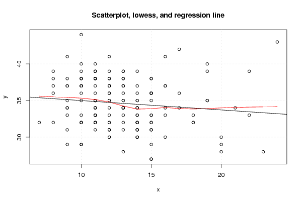
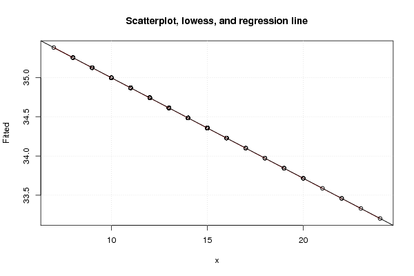
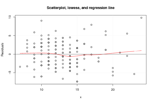
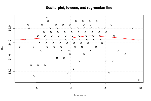
| Title produced by software | Linear Regression Graphical Model Validation | ||||||||||||||||||||||||||||||||||||||||||||||||||||||||||||
| Date of computation | Tue, 15 Nov 2011 12:30:14 -0500 | ||||||||||||||||||||||||||||||||||||||||||||||||||||||||||||
| Cite this page as follows | Statistical Computations at FreeStatistics.org, Office for Research Development and Education, URL https://freestatistics.org/blog/index.php?v=date/2011/Nov/15/t1321378252gkadwvrzhph2lfn.htm/, Retrieved Sat, 20 Apr 2024 11:19:00 +0000 | ||||||||||||||||||||||||||||||||||||||||||||||||||||||||||||
| Statistical Computations at FreeStatistics.org, Office for Research Development and Education, URL https://freestatistics.org/blog/index.php?pk=143251, Retrieved Sat, 20 Apr 2024 11:19:00 +0000 | |||||||||||||||||||||||||||||||||||||||||||||||||||||||||||||
| QR Codes: | |||||||||||||||||||||||||||||||||||||||||||||||||||||||||||||
|
| |||||||||||||||||||||||||||||||||||||||||||||||||||||||||||||
| Original text written by user: | |||||||||||||||||||||||||||||||||||||||||||||||||||||||||||||
| IsPrivate? | No (this computation is public) | ||||||||||||||||||||||||||||||||||||||||||||||||||||||||||||
| User-defined keywords | |||||||||||||||||||||||||||||||||||||||||||||||||||||||||||||
| Estimated Impact | 140 | ||||||||||||||||||||||||||||||||||||||||||||||||||||||||||||
Tree of Dependent Computations | |||||||||||||||||||||||||||||||||||||||||||||||||||||||||||||
| Family? (F = Feedback message, R = changed R code, M = changed R Module, P = changed Parameters, D = changed Data) | |||||||||||||||||||||||||||||||||||||||||||||||||||||||||||||
| - [Linear Regression Graphical Model Validation] [Colombia Coffee -...] [2008-02-26 10:22:06] [74be16979710d4c4e7c6647856088456] - M D [Linear Regression Graphical Model Validation] [ws6vb] [2010-11-13 11:31:05] [c7506ced21a6c0dca45d37c8a93c80e0] - D [Linear Regression Graphical Model Validation] [tt] [2010-11-13 12:51:28] [4a7069087cf9e0eda253aeed7d8c30d6] - D [Linear Regression Graphical Model Validation] [W6tutorial] [2010-11-13 14:33:02] [c7506ced21a6c0dca45d37c8a93c80e0] - D [Linear Regression Graphical Model Validation] [Workshop 6, Mini ...] [2010-11-14 15:39:04] [3635fb7041b1998c5a1332cf9de22bce] - R D [Linear Regression Graphical Model Validation] [Workshop 6: Mini-...] [2011-11-15 17:30:14] [e048104803f11a6160595af3ccdecef4] [Current] | |||||||||||||||||||||||||||||||||||||||||||||||||||||||||||||
| Feedback Forum | |||||||||||||||||||||||||||||||||||||||||||||||||||||||||||||
Post a new message | |||||||||||||||||||||||||||||||||||||||||||||||||||||||||||||
Dataset | |||||||||||||||||||||||||||||||||||||||||||||||||||||||||||||
| Dataseries X: | |||||||||||||||||||||||||||||||||||||||||||||||||||||||||||||
12 11 14 12 21 12 22 11 10 13 10 8 15 14 10 14 14 11 10 13 7 14 12 14 11 9 11 15 14 13 9 15 10 11 13 8 20 12 10 10 9 14 8 14 11 13 9 11 15 11 10 14 18 14 11 12 13 9 10 15 20 12 12 14 13 11 17 12 13 14 13 15 13 10 11 19 13 17 13 9 11 10 9 12 12 13 13 12 15 22 13 15 13 15 10 11 16 11 11 10 10 16 12 11 16 19 11 16 15 24 14 15 11 15 12 10 14 13 9 15 15 14 11 8 11 11 8 10 11 13 11 20 10 15 12 14 23 14 16 11 12 10 14 12 12 11 12 13 11 19 12 17 9 12 19 18 15 14 11 9 18 16 | |||||||||||||||||||||||||||||||||||||||||||||||||||||||||||||
| Dataseries Y: | |||||||||||||||||||||||||||||||||||||||||||||||||||||||||||||
41 39 30 31 34 35 39 34 36 37 38 36 38 39 33 32 36 38 39 32 32 31 39 37 39 41 36 33 33 34 31 27 37 34 34 32 29 36 29 35 37 34 38 35 38 37 38 33 36 38 32 32 32 34 32 37 39 29 37 35 30 38 34 31 34 35 36 30 39 35 38 31 34 38 34 39 37 34 28 37 33 37 35 37 32 33 38 33 29 33 31 36 35 32 29 39 37 35 37 32 38 37 36 32 33 40 38 41 36 43 30 31 32 32 37 37 33 34 33 38 33 31 38 37 33 31 39 44 33 35 32 28 40 27 37 32 28 34 30 35 31 32 30 30 31 40 32 36 32 35 38 42 34 35 35 33 36 32 33 34 32 34 | |||||||||||||||||||||||||||||||||||||||||||||||||||||||||||||
Tables (Output of Computation) | |||||||||||||||||||||||||||||||||||||||||||||||||||||||||||||
| |||||||||||||||||||||||||||||||||||||||||||||||||||||||||||||
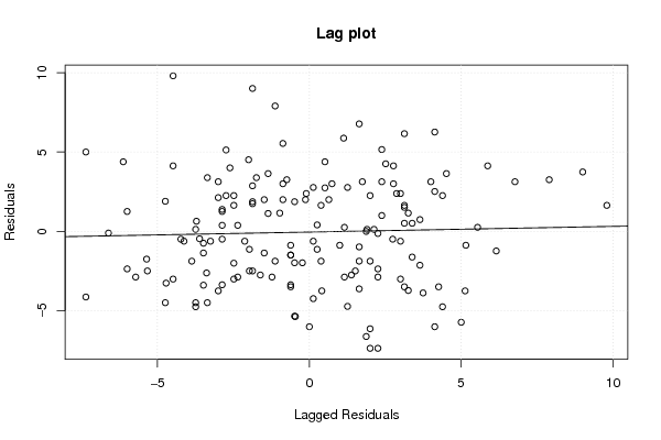
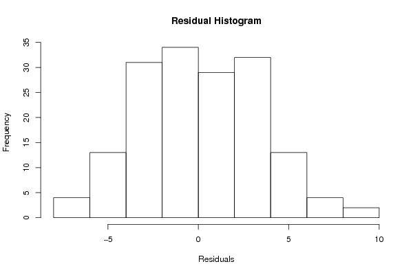
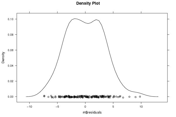
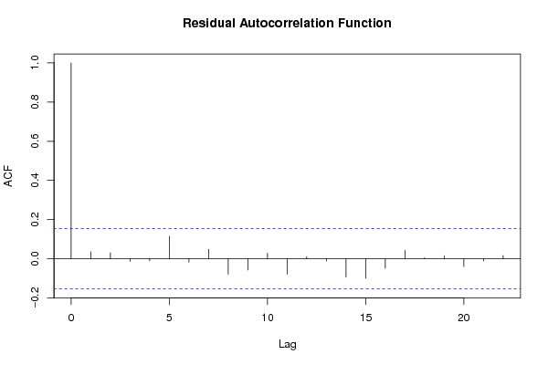
Figures (Output of Computation) | |||||||||||||||||||||||||||||||||||||||||||||||||||||||||||||
Input Parameters & R Code | |||||||||||||||||||||||||||||||||||||||||||||||||||||||||||||
| Parameters (Session): | |||||||||||||||||||||||||||||||||||||||||||||||||||||||||||||
| par1 = 0 ; | |||||||||||||||||||||||||||||||||||||||||||||||||||||||||||||
| Parameters (R input): | |||||||||||||||||||||||||||||||||||||||||||||||||||||||||||||
| par1 = 0 ; | |||||||||||||||||||||||||||||||||||||||||||||||||||||||||||||
| R code (references can be found in the software module): | |||||||||||||||||||||||||||||||||||||||||||||||||||||||||||||
par1 <- as.numeric(par1) | |||||||||||||||||||||||||||||||||||||||||||||||||||||||||||||