Free Statistics
of Irreproducible Research!
Description of Statistical Computation | |||||||||||||||||||||||||||||||||||||||||||||||||||||||||||||
|---|---|---|---|---|---|---|---|---|---|---|---|---|---|---|---|---|---|---|---|---|---|---|---|---|---|---|---|---|---|---|---|---|---|---|---|---|---|---|---|---|---|---|---|---|---|---|---|---|---|---|---|---|---|---|---|---|---|---|---|---|---|
| Author's title | |||||||||||||||||||||||||||||||||||||||||||||||||||||||||||||
| Author | *Unverified author* | ||||||||||||||||||||||||||||||||||||||||||||||||||||||||||||
| R Software Module | rwasp_linear_regression.wasp | ||||||||||||||||||||||||||||||||||||||||||||||||||||||||||||
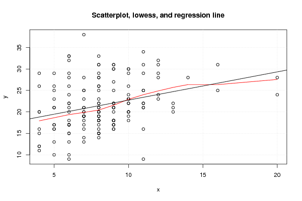
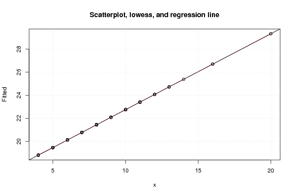
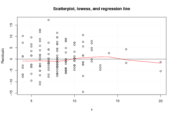
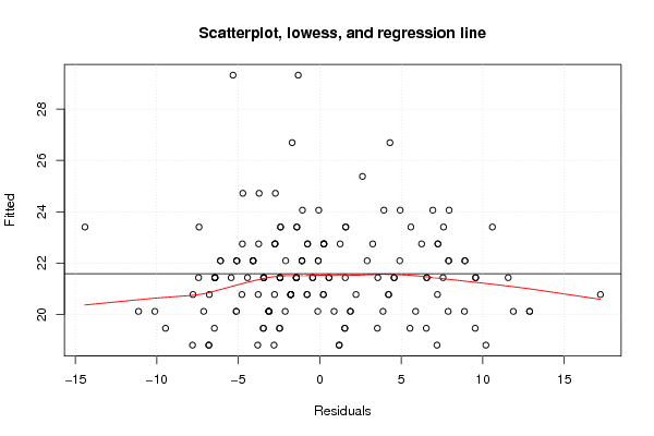
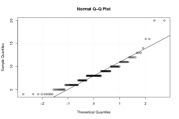
| Title produced by software | Linear Regression Graphical Model Validation | ||||||||||||||||||||||||||||||||||||||||||||||||||||||||||||
| Date of computation | Tue, 15 Nov 2011 11:49:20 -0500 | ||||||||||||||||||||||||||||||||||||||||||||||||||||||||||||
| Cite this page as follows | Statistical Computations at FreeStatistics.org, Office for Research Development and Education, URL https://freestatistics.org/blog/index.php?v=date/2011/Nov/15/t13213757835ishinx82t1yinj.htm/, Retrieved Sun, 13 Jul 2025 02:29:07 +0000 | ||||||||||||||||||||||||||||||||||||||||||||||||||||||||||||
| Statistical Computations at FreeStatistics.org, Office for Research Development and Education, URL https://freestatistics.org/blog/index.php?pk=143191, Retrieved Sun, 13 Jul 2025 02:29:07 +0000 | |||||||||||||||||||||||||||||||||||||||||||||||||||||||||||||
| QR Codes: | |||||||||||||||||||||||||||||||||||||||||||||||||||||||||||||
|
| |||||||||||||||||||||||||||||||||||||||||||||||||||||||||||||
| Original text written by user: | |||||||||||||||||||||||||||||||||||||||||||||||||||||||||||||
| IsPrivate? | No (this computation is public) | ||||||||||||||||||||||||||||||||||||||||||||||||||||||||||||
| User-defined keywords | |||||||||||||||||||||||||||||||||||||||||||||||||||||||||||||
| Estimated Impact | 258 | ||||||||||||||||||||||||||||||||||||||||||||||||||||||||||||
Tree of Dependent Computations | |||||||||||||||||||||||||||||||||||||||||||||||||||||||||||||
| Family? (F = Feedback message, R = changed R code, M = changed R Module, P = changed Parameters, D = changed Data) | |||||||||||||||||||||||||||||||||||||||||||||||||||||||||||||
| - [Linear Regression Graphical Model Validation] [Workshop 6 - Mini...] [2010-11-15 18:34:24] [74be16979710d4c4e7c6647856088456] - D [Linear Regression Graphical Model Validation] [Workshop 6 - mini...] [2010-11-15 18:55:36] [74be16979710d4c4e7c6647856088456] - D [Linear Regression Graphical Model Validation] [Workshop 6 - Mini...] [2010-11-15 19:17:39] [74be16979710d4c4e7c6647856088456] - D [Linear Regression Graphical Model Validation] [Mini-tutorial Hyp...] [2010-11-16 18:00:55] [a9e130f95bad0a0597234e75c6380c5a] - R P [Linear Regression Graphical Model Validation] [WS 6 - Mini-tutorial] [2011-11-15 16:49:20] [d41d8cd98f00b204e9800998ecf8427e] [Current] - M [Linear Regression Graphical Model Validation] [] [2011-11-15 19:17:30] [97a82ed57455ec27012f2e899dc4f1a4] - M [Linear Regression Graphical Model Validation] [] [2011-11-15 19:18:44] [97a82ed57455ec27012f2e899dc4f1a4] - M [Linear Regression Graphical Model Validation] [] [2011-11-15 19:36:09] [97a82ed57455ec27012f2e899dc4f1a4] | |||||||||||||||||||||||||||||||||||||||||||||||||||||||||||||
| Feedback Forum | |||||||||||||||||||||||||||||||||||||||||||||||||||||||||||||
Post a new message | |||||||||||||||||||||||||||||||||||||||||||||||||||||||||||||
Dataset | |||||||||||||||||||||||||||||||||||||||||||||||||||||||||||||
| Dataseries X: | |||||||||||||||||||||||||||||||||||||||||||||||||||||||||||||
12 8 8 8 9 7 4 11 7 7 12 10 10 8 8 4 9 8 7 11 9 11 13 8 8 9 6 9 9 6 6 16 5 7 9 6 6 5 12 7 10 9 8 5 8 8 10 6 8 7 4 8 8 4 20 8 8 6 4 8 9 6 7 9 5 5 8 8 6 8 7 7 9 11 6 8 6 9 8 6 10 8 8 10 5 7 5 8 14 7 8 6 5 6 10 12 9 12 7 8 10 6 10 10 10 5 7 10 11 6 7 12 11 11 11 5 8 6 9 4 4 7 11 6 7 8 4 8 9 8 11 8 5 4 8 10 6 9 9 13 9 10 20 5 11 6 9 7 9 10 9 8 7 6 13 6 8 10 16 | |||||||||||||||||||||||||||||||||||||||||||||||||||||||||||||
| Dataseries Y: | |||||||||||||||||||||||||||||||||||||||||||||||||||||||||||||
24 25 17 18 18 16 20 16 18 17 23 30 23 18 15 12 21 15 20 31 27 34 21 31 19 16 20 21 22 17 24 25 26 25 17 32 33 13 32 25 29 22 18 17 20 15 20 33 29 23 26 18 20 11 28 26 22 17 12 14 17 21 19 18 10 29 31 19 9 20 28 19 30 29 26 23 13 21 19 28 23 18 21 20 23 21 21 15 28 19 26 10 16 22 19 31 31 29 19 22 23 15 20 18 23 25 21 24 25 17 13 28 21 25 9 16 19 17 25 20 29 14 22 15 19 20 15 20 18 33 22 16 17 16 21 26 18 18 17 22 30 30 24 21 21 29 31 20 16 22 20 28 38 22 20 17 28 22 31 | |||||||||||||||||||||||||||||||||||||||||||||||||||||||||||||
Tables (Output of Computation) | |||||||||||||||||||||||||||||||||||||||||||||||||||||||||||||
| |||||||||||||||||||||||||||||||||||||||||||||||||||||||||||||
Figures (Output of Computation) | |||||||||||||||||||||||||||||||||||||||||||||||||||||||||||||
Input Parameters & R Code | |||||||||||||||||||||||||||||||||||||||||||||||||||||||||||||
| Parameters (Session): | |||||||||||||||||||||||||||||||||||||||||||||||||||||||||||||
| par1 = 0 ; par2 = 2 ; par3 = Pearson Chi-Squared ; | |||||||||||||||||||||||||||||||||||||||||||||||||||||||||||||
| Parameters (R input): | |||||||||||||||||||||||||||||||||||||||||||||||||||||||||||||
| par1 = 0 ; | |||||||||||||||||||||||||||||||||||||||||||||||||||||||||||||
| R code (references can be found in the software module): | |||||||||||||||||||||||||||||||||||||||||||||||||||||||||||||
par1 <- as.numeric(par1) | |||||||||||||||||||||||||||||||||||||||||||||||||||||||||||||