Free Statistics
of Irreproducible Research!
Description of Statistical Computation | |||||||||||||||||||||||||||||||||||||||||||||||||||||||||||||
|---|---|---|---|---|---|---|---|---|---|---|---|---|---|---|---|---|---|---|---|---|---|---|---|---|---|---|---|---|---|---|---|---|---|---|---|---|---|---|---|---|---|---|---|---|---|---|---|---|---|---|---|---|---|---|---|---|---|---|---|---|---|
| Author's title | |||||||||||||||||||||||||||||||||||||||||||||||||||||||||||||
| Author | *The author of this computation has been verified* | ||||||||||||||||||||||||||||||||||||||||||||||||||||||||||||
| R Software Module | rwasp_linear_regression.wasp | ||||||||||||||||||||||||||||||||||||||||||||||||||||||||||||
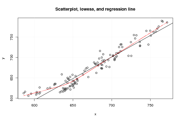
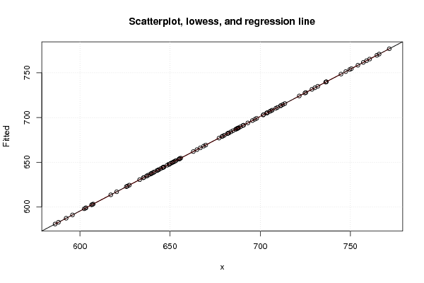
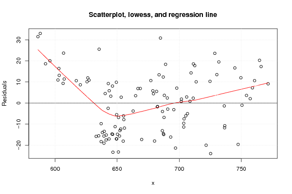
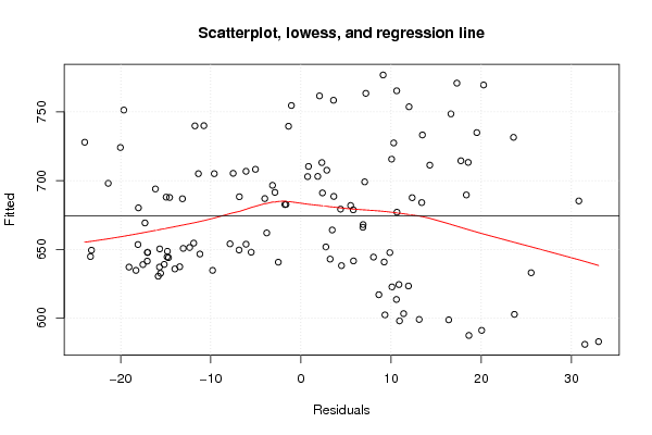
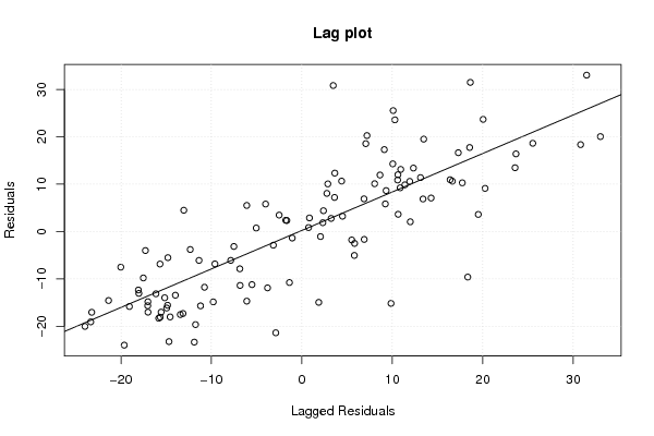
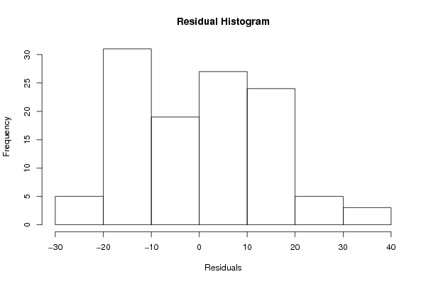
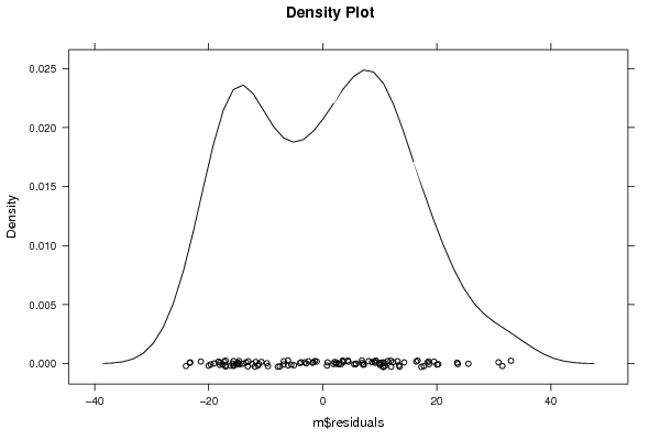
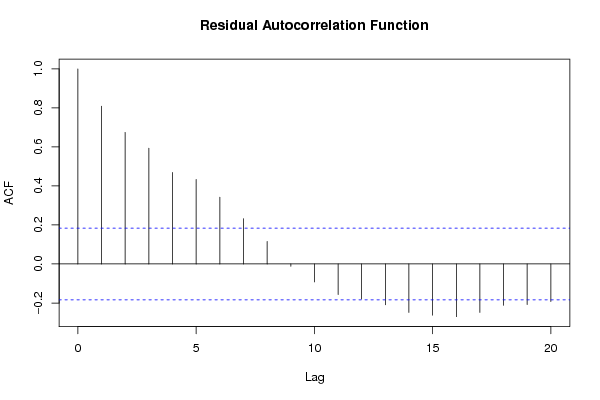
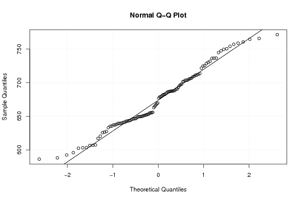
| Title produced by software | Linear Regression Graphical Model Validation | ||||||||||||||||||||||||||||||||||||||||||||||||||||||||||||
| Date of computation | Tue, 15 Nov 2011 10:26:29 -0500 | ||||||||||||||||||||||||||||||||||||||||||||||||||||||||||||
| Cite this page as follows | Statistical Computations at FreeStatistics.org, Office for Research Development and Education, URL https://freestatistics.org/blog/index.php?v=date/2011/Nov/15/t1321370887lgxjl9id91ohux9.htm/, Retrieved Tue, 16 Apr 2024 07:28:00 +0000 | ||||||||||||||||||||||||||||||||||||||||||||||||||||||||||||
| Statistical Computations at FreeStatistics.org, Office for Research Development and Education, URL https://freestatistics.org/blog/index.php?pk=143052, Retrieved Tue, 16 Apr 2024 07:28:00 +0000 | |||||||||||||||||||||||||||||||||||||||||||||||||||||||||||||
| QR Codes: | |||||||||||||||||||||||||||||||||||||||||||||||||||||||||||||
|
| |||||||||||||||||||||||||||||||||||||||||||||||||||||||||||||
| Original text written by user: | |||||||||||||||||||||||||||||||||||||||||||||||||||||||||||||
| IsPrivate? | No (this computation is public) | ||||||||||||||||||||||||||||||||||||||||||||||||||||||||||||
| User-defined keywords | |||||||||||||||||||||||||||||||||||||||||||||||||||||||||||||
| Estimated Impact | 98 | ||||||||||||||||||||||||||||||||||||||||||||||||||||||||||||
Tree of Dependent Computations | |||||||||||||||||||||||||||||||||||||||||||||||||||||||||||||
| Family? (F = Feedback message, R = changed R code, M = changed R Module, P = changed Parameters, D = changed Data) | |||||||||||||||||||||||||||||||||||||||||||||||||||||||||||||
| - [Linear Regression Graphical Model Validation] [Colombia Coffee -...] [2008-02-26 10:22:06] [74be16979710d4c4e7c6647856088456] - RM D [Linear Regression Graphical Model Validation] [Linear regression...] [2011-11-13 10:41:52] [74be16979710d4c4e7c6647856088456] - [Linear Regression Graphical Model Validation] [WS 6-Opdracht 2B] [2011-11-15 08:27:38] [570fce4db58fd7864ac807c4286d6e49] - D [Linear Regression Graphical Model Validation] [Mini-tutorial: Li...] [2011-11-15 14:45:07] [570fce4db58fd7864ac807c4286d6e49] - R D [Linear Regression Graphical Model Validation] [WS 6 lineair verband] [2011-11-15 15:26:29] [080b56dea5ee02335c893a05354948d0] [Current] | |||||||||||||||||||||||||||||||||||||||||||||||||||||||||||||
| Feedback Forum | |||||||||||||||||||||||||||||||||||||||||||||||||||||||||||||
Post a new message | |||||||||||||||||||||||||||||||||||||||||||||||||||||||||||||
Dataset | |||||||||||||||||||||||||||||||||||||||||||||||||||||||||||||
| Dataseries X: | |||||||||||||||||||||||||||||||||||||||||||||||||||||||||||||
637.12 633.12 639.38 646.62 655.88 662.88 652.88 654.88 651.88 643.5 651 645.88 655.12 655.38 651.12 639.38 648.38 649.62 650.25 649.38 649.62 635.12 646.38 637.12 641.12 639.62 638.12 641.25 649.38 607.38 603.38 602.38 603.12 606.88 595.88 588.12 586.25 592.38 635.5 625.75 646.25 653.25 644.88 640.38 652.25 680.12 687.25 697 690.75 695.62 703.88 721.62 725.25 747.38 736.5 736.62 736.25 750.5 757.12 749.62 760.62 744.75 765.88 771.5 764.62 758.88 754.12 731.88 730.25 728.62 724.75 712.5 711.38 698 709.5 713.62 706 708.62 701.62 706.62 678.75 686.5 669.75 686.38 693.12 687.5 701.75 711.25 682.5 668.62 666.75 683.75 687.12 688 677.12 679.25 690.38 682.38 681.75 705.25 703.62 687.75 703.62 689 684.88 664.88 642.75 643.62 642.88 627.38 617.12 626.38 620.38 606.5 | |||||||||||||||||||||||||||||||||||||||||||||||||||||||||||||
| Dataseries Y: | |||||||||||||||||||||||||||||||||||||||||||||||||||||||||||||
616.38 614.62 618 621.38 642.62 658.12 639 635.38 634.62 624.38 626.12 629.25 647.62 646.12 642.62 621.38 635.38 642.38 633.75 630.62 630.88 617 629.62 624.88 621.38 623.88 621.75 623.88 657.5 614.62 612.12 608.88 615.12 626.38 611.12 615.88 612.38 606 658.5 632.75 652.38 654.5 646.12 642.62 637.62 662.12 673.12 676.62 688.5 693.38 697.75 704 703.88 731.62 728 729.12 738.12 753.5 763.62 765.62 775.88 765.12 788.12 785.88 789.75 770.62 762 754.38 746.62 755 737.62 732.12 731.75 706.12 725.5 725.62 710.38 711.12 703.62 703.12 684.5 682.88 651.88 673.62 677.75 673 704.88 715.38 681 674.88 672.88 697.38 699.88 692.12 687.62 683.62 693.38 680.75 687.38 700.62 693.62 681.38 695.38 707.88 716 667.5 638.12 647.38 650 635.25 624.12 635.25 625.62 611.62 | |||||||||||||||||||||||||||||||||||||||||||||||||||||||||||||
Tables (Output of Computation) | |||||||||||||||||||||||||||||||||||||||||||||||||||||||||||||
| |||||||||||||||||||||||||||||||||||||||||||||||||||||||||||||
Figures (Output of Computation) | |||||||||||||||||||||||||||||||||||||||||||||||||||||||||||||
Input Parameters & R Code | |||||||||||||||||||||||||||||||||||||||||||||||||||||||||||||
| Parameters (Session): | |||||||||||||||||||||||||||||||||||||||||||||||||||||||||||||
| par1 = 0 ; | |||||||||||||||||||||||||||||||||||||||||||||||||||||||||||||
| Parameters (R input): | |||||||||||||||||||||||||||||||||||||||||||||||||||||||||||||
| par1 = 0 ; | |||||||||||||||||||||||||||||||||||||||||||||||||||||||||||||
| R code (references can be found in the software module): | |||||||||||||||||||||||||||||||||||||||||||||||||||||||||||||
par1 <- as.numeric(par1) | |||||||||||||||||||||||||||||||||||||||||||||||||||||||||||||