Free Statistics
of Irreproducible Research!
Description of Statistical Computation | |||||||||||||||||||||
|---|---|---|---|---|---|---|---|---|---|---|---|---|---|---|---|---|---|---|---|---|---|
| Author's title | |||||||||||||||||||||
| Author | *The author of this computation has been verified* | ||||||||||||||||||||
| R Software Module | rwasp_meanplot.wasp | ||||||||||||||||||||
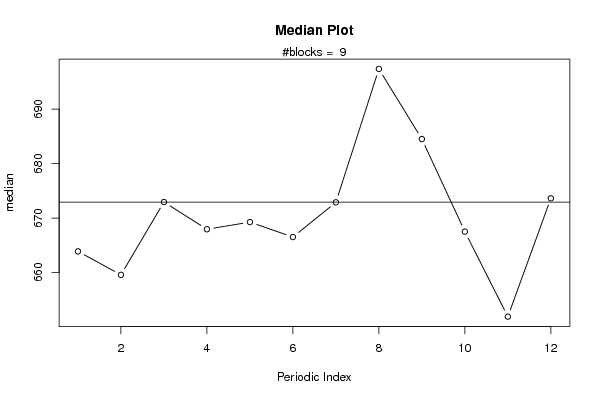
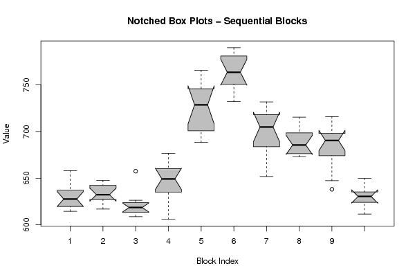
| Title produced by software | Mean Plot | ||||||||||||||||||||
| Date of computation | Tue, 15 Nov 2011 09:49:30 -0500 | ||||||||||||||||||||
| Cite this page as follows | Statistical Computations at FreeStatistics.org, Office for Research Development and Education, URL https://freestatistics.org/blog/index.php?v=date/2011/Nov/15/t1321368599b6syb2rhq1fc5mp.htm/, Retrieved Fri, 19 Apr 2024 18:21:44 +0000 | ||||||||||||||||||||
| Statistical Computations at FreeStatistics.org, Office for Research Development and Education, URL https://freestatistics.org/blog/index.php?pk=142968, Retrieved Fri, 19 Apr 2024 18:21:44 +0000 | |||||||||||||||||||||
| QR Codes: | |||||||||||||||||||||
|
| |||||||||||||||||||||
| Original text written by user: | |||||||||||||||||||||
| IsPrivate? | No (this computation is public) | ||||||||||||||||||||
| User-defined keywords | |||||||||||||||||||||
| Estimated Impact | 93 | ||||||||||||||||||||
Tree of Dependent Computations | |||||||||||||||||||||
| Family? (F = Feedback message, R = changed R code, M = changed R Module, P = changed Parameters, D = changed Data) | |||||||||||||||||||||
| - [Bivariate Data Series] [Bivariate dataset] [2008-01-05 23:51:08] [74be16979710d4c4e7c6647856088456] - RMPD [Blocked Bootstrap Plot - Central Tendency] [Colombia Coffee] [2008-01-07 10:26:26] [74be16979710d4c4e7c6647856088456] - M D [Blocked Bootstrap Plot - Central Tendency] [WS 6 - tweede opd...] [2011-11-14 21:10:39] [570fce4db58fd7864ac807c4286d6e49] - D [Blocked Bootstrap Plot - Central Tendency] [Mini-tutorial: No...] [2011-11-15 11:58:10] [570fce4db58fd7864ac807c4286d6e49] - RMPD [Mean Plot] [WS 6 boxplot Mais] [2011-11-15 14:48:22] [10b12745961ee885a66356b3bf31ed40] - D [Mean Plot] [WS 6 boxplot Graan] [2011-11-15 14:49:30] [080b56dea5ee02335c893a05354948d0] [Current] | |||||||||||||||||||||
| Feedback Forum | |||||||||||||||||||||
Post a new message | |||||||||||||||||||||
Dataset | |||||||||||||||||||||
| Dataseries X: | |||||||||||||||||||||
616.38 614.62 618 621.38 642.62 658.12 639 635.38 634.62 624.38 626.12 629.25 647.62 646.12 642.62 621.38 635.38 642.38 633.75 630.62 630.88 617 629.62 624.88 621.38 623.88 621.75 623.88 657.5 614.62 612.12 608.88 615.12 626.38 611.12 615.88 612.38 606 658.5 632.75 652.38 654.5 646.12 642.62 637.62 662.12 673.12 676.62 688.5 693.38 697.75 704 703.88 731.62 728 729.12 738.12 753.5 763.62 765.62 775.88 765.12 788.12 785.88 789.75 770.62 762 754.38 746.62 755 737.62 732.12 731.75 706.12 725.5 725.62 710.38 711.12 703.62 703.12 684.5 682.88 651.88 673.62 677.75 673 704.88 715.38 681 674.88 672.88 697.38 699.88 692.12 687.62 683.62 693.38 680.75 687.38 700.62 693.62 681.38 695.38 707.88 716 667.5 638.12 647.38 650 635.25 624.12 635.25 625.62 611.62 | |||||||||||||||||||||
Tables (Output of Computation) | |||||||||||||||||||||
| |||||||||||||||||||||
Figures (Output of Computation) | |||||||||||||||||||||
Input Parameters & R Code | |||||||||||||||||||||
| Parameters (Session): | |||||||||||||||||||||
| par1 = 12 ; | |||||||||||||||||||||
| Parameters (R input): | |||||||||||||||||||||
| par1 = 12 ; | |||||||||||||||||||||
| R code (references can be found in the software module): | |||||||||||||||||||||
par1 <- as.numeric(par1) | |||||||||||||||||||||