Free Statistics
of Irreproducible Research!
Description of Statistical Computation | |||||||||||||||||||||
|---|---|---|---|---|---|---|---|---|---|---|---|---|---|---|---|---|---|---|---|---|---|
| Author's title | |||||||||||||||||||||
| Author | *The author of this computation has been verified* | ||||||||||||||||||||
| R Software Module | rwasp_meanplot.wasp | ||||||||||||||||||||
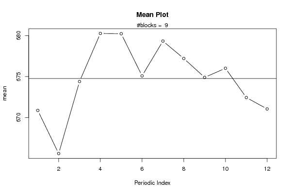
| Title produced by software | Mean Plot | ||||||||||||||||||||
| Date of computation | Tue, 15 Nov 2011 09:48:22 -0500 | ||||||||||||||||||||
| Cite this page as follows | Statistical Computations at FreeStatistics.org, Office for Research Development and Education, URL https://freestatistics.org/blog/index.php?v=date/2011/Nov/15/t1321368524eb2lten7e6v2soz.htm/, Retrieved Wed, 24 Apr 2024 21:25:42 +0000 | ||||||||||||||||||||
| Statistical Computations at FreeStatistics.org, Office for Research Development and Education, URL https://freestatistics.org/blog/index.php?pk=142965, Retrieved Wed, 24 Apr 2024 21:25:42 +0000 | |||||||||||||||||||||
| QR Codes: | |||||||||||||||||||||
|
| |||||||||||||||||||||
| Original text written by user: | |||||||||||||||||||||
| IsPrivate? | No (this computation is public) | ||||||||||||||||||||
| User-defined keywords | |||||||||||||||||||||
| Estimated Impact | 101 | ||||||||||||||||||||
Tree of Dependent Computations | |||||||||||||||||||||
| Family? (F = Feedback message, R = changed R code, M = changed R Module, P = changed Parameters, D = changed Data) | |||||||||||||||||||||
| - [Bivariate Data Series] [Bivariate dataset] [2008-01-05 23:51:08] [74be16979710d4c4e7c6647856088456] - RMPD [Blocked Bootstrap Plot - Central Tendency] [Colombia Coffee] [2008-01-07 10:26:26] [74be16979710d4c4e7c6647856088456] - M D [Blocked Bootstrap Plot - Central Tendency] [WS 6 - tweede opd...] [2011-11-14 21:10:39] [570fce4db58fd7864ac807c4286d6e49] - D [Blocked Bootstrap Plot - Central Tendency] [Mini-tutorial: No...] [2011-11-15 11:58:10] [570fce4db58fd7864ac807c4286d6e49] - RMPD [Mean Plot] [WS 6 boxplot Mais] [2011-11-15 14:48:22] [080b56dea5ee02335c893a05354948d0] [Current] - D [Mean Plot] [WS 6 boxplot Graan] [2011-11-15 14:49:30] [10b12745961ee885a66356b3bf31ed40] | |||||||||||||||||||||
| Feedback Forum | |||||||||||||||||||||
Post a new message | |||||||||||||||||||||
Dataset | |||||||||||||||||||||
| Dataseries X: | |||||||||||||||||||||
637.12 633.12 639.38 646.62 655.88 662.88 652.88 654.88 651.88 643.5 651 645.88 655.12 655.38 651.12 639.38 648.38 649.62 650.25 649.38 649.62 635.12 646.38 637.12 641.12 639.62 638.12 641.25 649.38 607.38 603.38 602.38 603.12 606.88 595.88 588.12 586.25 592.38 635.5 625.75 646.25 653.25 644.88 640.38 652.25 680.12 687.25 697 690.75 695.62 703.88 721.62 725.25 747.38 736.5 736.62 736.25 750.5 757.12 749.62 760.62 744.75 765.88 771.5 764.62 758.88 754.12 731.88 730.25 728.62 724.75 712.5 711.38 698 709.5 713.62 706 708.62 701.62 706.62 678.75 686.5 669.75 686.38 693.12 687.5 701.75 711.25 682.5 668.62 666.75 683.75 687.12 688 677.12 679.25 690.38 682.38 681.75 705.25 703.62 687.75 703.62 689 684.88 664.88 642.75 643.62 642.88 627.38 617.12 626.38 620.38 606.5 | |||||||||||||||||||||
Tables (Output of Computation) | |||||||||||||||||||||
| |||||||||||||||||||||
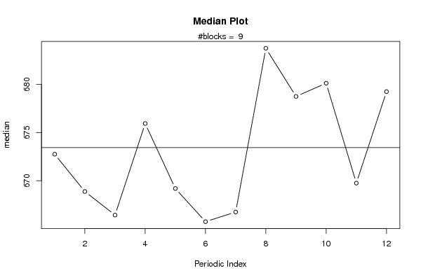
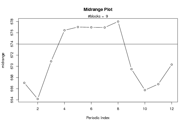
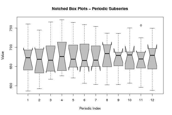
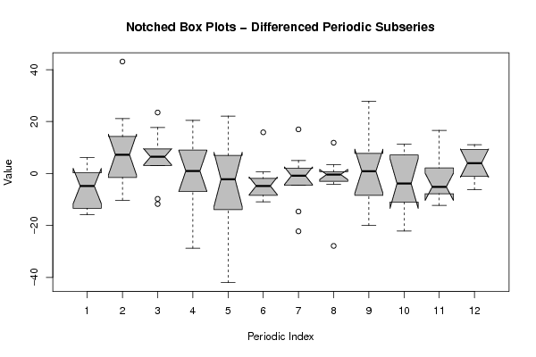
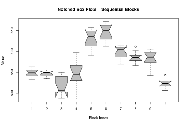
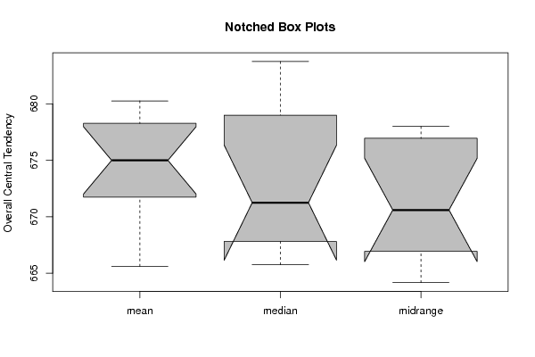
Figures (Output of Computation) | |||||||||||||||||||||
Input Parameters & R Code | |||||||||||||||||||||
| Parameters (Session): | |||||||||||||||||||||
| par1 = 12 ; | |||||||||||||||||||||
| Parameters (R input): | |||||||||||||||||||||
| par1 = 12 ; | |||||||||||||||||||||
| R code (references can be found in the software module): | |||||||||||||||||||||
par1 <- as.numeric(par1) | |||||||||||||||||||||