Free Statistics
of Irreproducible Research!
Description of Statistical Computation | |||||||||||||||||||||||||||||||||||||||||||||||||||||
|---|---|---|---|---|---|---|---|---|---|---|---|---|---|---|---|---|---|---|---|---|---|---|---|---|---|---|---|---|---|---|---|---|---|---|---|---|---|---|---|---|---|---|---|---|---|---|---|---|---|---|---|---|---|
| Author's title | |||||||||||||||||||||||||||||||||||||||||||||||||||||
| Author | *The author of this computation has been verified* | ||||||||||||||||||||||||||||||||||||||||||||||||||||
| R Software Module | rwasp_bidataseries.wasp | ||||||||||||||||||||||||||||||||||||||||||||||||||||
| Title produced by software | Bivariate Data Series | ||||||||||||||||||||||||||||||||||||||||||||||||||||
| Date of computation | Tue, 15 Nov 2011 06:08:11 -0500 | ||||||||||||||||||||||||||||||||||||||||||||||||||||
| Cite this page as follows | Statistical Computations at FreeStatistics.org, Office for Research Development and Education, URL https://freestatistics.org/blog/index.php?v=date/2011/Nov/15/t1321355303m3ll9qu8fmnqw28.htm/, Retrieved Thu, 25 Apr 2024 01:29:11 +0000 | ||||||||||||||||||||||||||||||||||||||||||||||||||||
| Statistical Computations at FreeStatistics.org, Office for Research Development and Education, URL https://freestatistics.org/blog/index.php?pk=142725, Retrieved Thu, 25 Apr 2024 01:29:11 +0000 | |||||||||||||||||||||||||||||||||||||||||||||||||||||
| QR Codes: | |||||||||||||||||||||||||||||||||||||||||||||||||||||
|
| |||||||||||||||||||||||||||||||||||||||||||||||||||||
| Original text written by user: | |||||||||||||||||||||||||||||||||||||||||||||||||||||
| IsPrivate? | No (this computation is public) | ||||||||||||||||||||||||||||||||||||||||||||||||||||
| User-defined keywords | |||||||||||||||||||||||||||||||||||||||||||||||||||||
| Estimated Impact | 86 | ||||||||||||||||||||||||||||||||||||||||||||||||||||
Tree of Dependent Computations | |||||||||||||||||||||||||||||||||||||||||||||||||||||
| Family? (F = Feedback message, R = changed R code, M = changed R Module, P = changed Parameters, D = changed Data) | |||||||||||||||||||||||||||||||||||||||||||||||||||||
| - [Bivariate Data Series] [Bivariate dataset] [2008-01-05 23:51:08] [74be16979710d4c4e7c6647856088456] - RMPD [Bivariate Data Series] [brandverzekering] [2011-11-15 11:08:11] [89a94f030b332f6008ade04d76806a4c] [Current] | |||||||||||||||||||||||||||||||||||||||||||||||||||||
| Feedback Forum | |||||||||||||||||||||||||||||||||||||||||||||||||||||
Post a new message | |||||||||||||||||||||||||||||||||||||||||||||||||||||
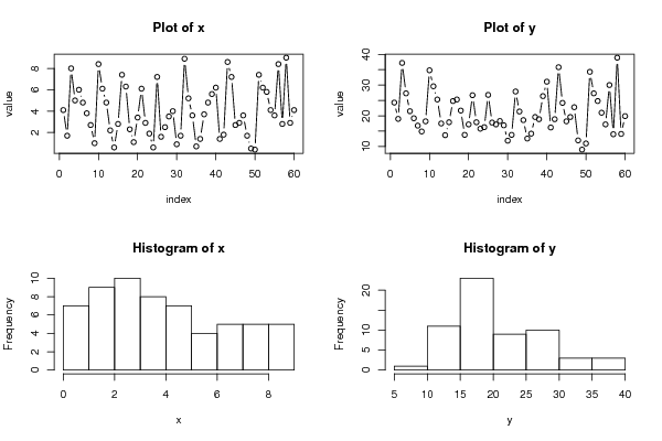
Dataset | |||||||||||||||||||||||||||||||||||||||||||||||||||||
| Dataseries X: | |||||||||||||||||||||||||||||||||||||||||||||||||||||
4.1 1.7 8 5 6 4.8 3.8 2.7 1 8.4 6.1 4.8 2.2 0.6 2.8 7.4 6.3 2.3 1.1 3.4 6.1 2.9 1.9 0.6 7.2 1.6 2.5 3.5 4 0.9 1.7 8.9 5.2 3.6 0.7 1.4 3.7 4.8 5.6 6.2 1.4 1.8 8.6 7.2 2.7 2.9 3.6 1.7 0.5 0.4 7.4 6.2 5.8 4.1 3.6 8.4 2.8 9 2.9 4.1 | |||||||||||||||||||||||||||||||||||||||||||||||||||||
| Dataseries Y: | |||||||||||||||||||||||||||||||||||||||||||||||||||||
24.3 19 37.2 27.3 21.5 19.2 16.8 14.9 18.2 34.8 29.6 25.3 17.5 13.7 17.9 24.8 25.3 21.7 13.8 17.2 26.7 17.9 15.8 16.3 26.8 17.8 17.2 18.3 16.9 11.9 13.8 27.9 21.4 18.6 12.6 14.2 19.6 18.9 26.4 31.1 16.2 18.9 35.8 24.2 18.2 19.6 22.8 12 9 11 34.3 27.3 24.8 21 17.2 30 14 38.9 14.1 19.9 | |||||||||||||||||||||||||||||||||||||||||||||||||||||
Tables (Output of Computation) | |||||||||||||||||||||||||||||||||||||||||||||||||||||
| |||||||||||||||||||||||||||||||||||||||||||||||||||||
Figures (Output of Computation) | |||||||||||||||||||||||||||||||||||||||||||||||||||||
Input Parameters & R Code | |||||||||||||||||||||||||||||||||||||||||||||||||||||
| Parameters (Session): | |||||||||||||||||||||||||||||||||||||||||||||||||||||
| par1 = 3 ; par2 = 4 ; par3 = Pearson Chi-Squared ; | |||||||||||||||||||||||||||||||||||||||||||||||||||||
| Parameters (R input): | |||||||||||||||||||||||||||||||||||||||||||||||||||||
| par1 = afstand ; par2 = www.ico.org ; par3 = Prices paid to growers in exporting Member countries in US cents per lb (Arabica, 1977/1 - 2006/12) ; par4 = bedrag ; par5 = www.ico.org ; par6 = Retail prices in importing Member countries in US cents per lb (Arabica, 1977/1 - 2006/12) ; | |||||||||||||||||||||||||||||||||||||||||||||||||||||
| R code (references can be found in the software module): | |||||||||||||||||||||||||||||||||||||||||||||||||||||
bitmap(file='test1.png') | |||||||||||||||||||||||||||||||||||||||||||||||||||||