Free Statistics
of Irreproducible Research!
Description of Statistical Computation | |||||||||||||||||||||||||||||||||||||||||||||||||||||||||||||
|---|---|---|---|---|---|---|---|---|---|---|---|---|---|---|---|---|---|---|---|---|---|---|---|---|---|---|---|---|---|---|---|---|---|---|---|---|---|---|---|---|---|---|---|---|---|---|---|---|---|---|---|---|---|---|---|---|---|---|---|---|---|
| Author's title | |||||||||||||||||||||||||||||||||||||||||||||||||||||||||||||
| Author | *The author of this computation has been verified* | ||||||||||||||||||||||||||||||||||||||||||||||||||||||||||||
| R Software Module | rwasp_linear_regression.wasp | ||||||||||||||||||||||||||||||||||||||||||||||||||||||||||||
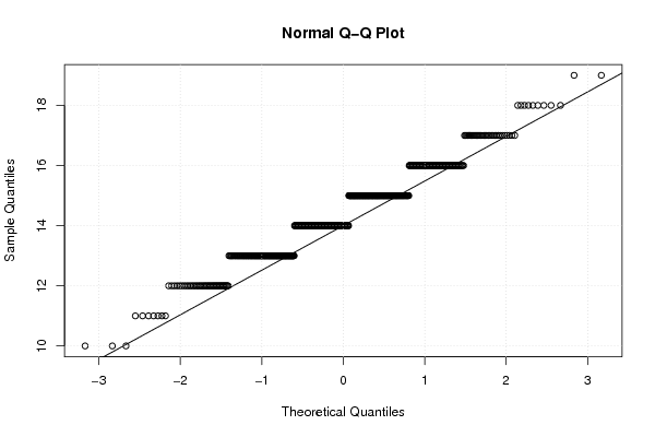
| Title produced by software | Linear Regression Graphical Model Validation | ||||||||||||||||||||||||||||||||||||||||||||||||||||||||||||
| Date of computation | Tue, 15 Nov 2011 05:25:29 -0500 | ||||||||||||||||||||||||||||||||||||||||||||||||||||||||||||
| Cite this page as follows | Statistical Computations at FreeStatistics.org, Office for Research Development and Education, URL https://freestatistics.org/blog/index.php?v=date/2011/Nov/15/t13213527506vwkp3sbxdrvbp9.htm/, Retrieved Fri, 19 Apr 2024 14:30:14 +0000 | ||||||||||||||||||||||||||||||||||||||||||||||||||||||||||||
| Statistical Computations at FreeStatistics.org, Office for Research Development and Education, URL https://freestatistics.org/blog/index.php?pk=142661, Retrieved Fri, 19 Apr 2024 14:30:14 +0000 | |||||||||||||||||||||||||||||||||||||||||||||||||||||||||||||
| QR Codes: | |||||||||||||||||||||||||||||||||||||||||||||||||||||||||||||
|
| |||||||||||||||||||||||||||||||||||||||||||||||||||||||||||||
| Original text written by user: | |||||||||||||||||||||||||||||||||||||||||||||||||||||||||||||
| IsPrivate? | No (this computation is public) | ||||||||||||||||||||||||||||||||||||||||||||||||||||||||||||
| User-defined keywords | Hypothese 3 | ||||||||||||||||||||||||||||||||||||||||||||||||||||||||||||
| Estimated Impact | 93 | ||||||||||||||||||||||||||||||||||||||||||||||||||||||||||||
Tree of Dependent Computations | |||||||||||||||||||||||||||||||||||||||||||||||||||||||||||||
| Family? (F = Feedback message, R = changed R code, M = changed R Module, P = changed Parameters, D = changed Data) | |||||||||||||||||||||||||||||||||||||||||||||||||||||||||||||
| - [Linear Regression Graphical Model Validation] [Colombia Coffee -...] [2008-02-26 10:22:06] [74be16979710d4c4e7c6647856088456] - M D [Linear Regression Graphical Model Validation] [mini-tutorial] [2011-11-15 10:25:29] [065e524ef27b3ebe8baf73e00eb8c266] [Current] | |||||||||||||||||||||||||||||||||||||||||||||||||||||||||||||
| Feedback Forum | |||||||||||||||||||||||||||||||||||||||||||||||||||||||||||||
Post a new message | |||||||||||||||||||||||||||||||||||||||||||||||||||||||||||||
Dataset | |||||||||||||||||||||||||||||||||||||||||||||||||||||||||||||
| Dataseries X: | |||||||||||||||||||||||||||||||||||||||||||||||||||||||||||||
14 13 16 13 14 15 14 13 15 13 13 13 16 16 12 15 16 16 12 16 13 14 11 12 15 15 14 15 15 15 16 15 16 12 16 12 18 18 15 17 17 16 14 14 15 14 14 17 15 14 15 14 15 15 14 15 14 16 15 15 14 16 16 13 13 15 14 13 17 18 13 16 13 15 15 13 14 14 14 15 12 16 13 15 16 14 17 12 16 13 13 14 14 13 15 15 15 12 12 14 12 15 14 15 13 15 14 13 14 14 17 14 12 15 16 16 13 14 15 13 17 13 13 12 14 15 13 15 13 15 14 16 13 15 15 14 13 15 16 15 16 16 16 14 12 13 15 15 15 14 14 14 13 15 13 15 16 15 13 13 14 15 15 16 15 12 14 16 14 14 14 12 18 14 16 12 14 13 14 16 13 13 13 14 13 14 14 14 15 15 14 13 14 17 13 15 14 16 14 14 14 17 13 14 15 18 15 15 16 15 15 12 14 14 15 14 17 15 14 13 14 14 13 14 14 14 14 15 14 15 13 12 14 14 14 15 15 15 13 13 13 14 13 12 14 15 15 10 14 14 18 15 12 13 17 14 16 14 17 15 19 13 17 16 15 15 14 14 14 12 16 17 14 13 14 13 18 14 12 15 14 16 13 15 16 13 15 13 13 12 14 15 14 15 15 15 14 15 13 13 17 13 11 16 13 15 13 14 15 15 13 15 13 13 14 14 16 15 15 15 16 13 14 15 13 17 13 12 13 15 12 12 14 13 13 15 14 13 17 13 16 16 13 14 13 12 15 15 16 13 13 15 14 15 15 16 14 13 13 15 15 13 11 13 16 13 13 15 15 14 12 14 15 13 13 14 15 16 13 16 13 16 16 14 13 14 14 14 15 14 16 15 14 13 12 16 13 13 13 12 14 12 13 15 15 13 14 13 14 16 16 15 16 15 13 13 16 14 14 14 11 14 14 13 15 12 14 15 15 15 16 19 16 14 13 16 12 16 15 11 16 16 15 15 17 15 14 13 14 16 14 14 17 14 15 15 14 14 16 13 15 14 14 16 15 14 17 16 15 13 15 14 10 15 14 16 14 15 15 15 14 17 15 15 15 15 16 13 15 16 13 17 12 15 15 17 13 17 13 15 15 14 16 15 16 14 17 14 16 16 15 13 15 14 14 15 17 16 15 15 14 14 14 13 14 16 14 16 13 13 16 15 16 14 12 15 14 15 14 17 13 14 15 15 15 15 15 16 17 16 14 13 14 16 16 14 14 15 13 15 17 14 10 14 15 15 15 12 16 14 16 15 13 13 12 13 17 18 15 15 12 14 13 14 15 16 14 15 17 18 15 14 15 12 12 13 15 13 11 15 14 14 16 13 15 13 13 14 12 15 13 15 14 16 15 14 14 16 15 17 14 14 16 15 13 15 11 16 14 15 16 13 13 14 15 14 14 15 13 13 13 17 14 17 14 16 15 16 12 16 15 15 15 | |||||||||||||||||||||||||||||||||||||||||||||||||||||||||||||
| Dataseries Y: | |||||||||||||||||||||||||||||||||||||||||||||||||||||||||||||
96 91 108 95 105 117 94 98 120 91 100 90 123 97 120 133 141 138 85 121 74 100 67 73 116 115 92 109 120 105 115 105 122 87 94 78 135 113 123 126 127 120 108 83 117 96 103 134 112 93 103 84 116 97 87 122 111 101 109 96 100 90 120 86 85 96 93 95 127 156 94 123 80 98 88 109 98 83 85 85 76 96 72 125 121 103 113 89 108 80 87 84 93 94 87 95 106 94 91 106 103 121 112 98 91 112 118 90 80 73 135 97 82 99 132 130 67 78 131 80 121 79 82 101 91 83 76 93 73 107 97 133 74 93 99 105 95 90 115 95 115 105 115 102 92 101 90 93 102 79 83 89 65 97 78 99 126 106 115 90 104 76 95 114 81 91 120 132 96 95 74 93 152 116 148 84 87 114 106 110 99 96 80 144 102 125 98 87 100 128 102 104 96 127 85 106 85 126 121 94 94 128 82 118 128 149 92 105 146 106 130 77 92 83 88 89 132 113 83 84 88 74 71 119 120 113 88 92 91 123 80 79 109 98 98 106 117 108 79 93 86 106 100 78 92 111 97 77 134 95 134 96 78 79 87 95 110 96 129 93 154 97 109 118 91 83 65 99 103 75 135 109 98 81 78 75 171 96 78 96 121 100 97 99 92 108 96 77 82 94 98 139 116 126 121 96 91 99 74 95 118 74 96 117 85 84 100 88 120 97 94 105 81 70 83 93 141 109 115 97 109 103 95 92 80 109 86 74 84 121 99 76 73 73 66 134 102 81 144 78 95 116 118 77 77 72 113 104 111 86 76 117 103 95 87 105 84 90 90 84 109 113 73 102 124 102 78 103 122 112 76 97 95 106 77 88 85 121 86 113 95 92 97 83 81 90 89 83 89 90 110 116 95 79 87 109 90 96 81 93 101 80 90 108 102 90 93 97 128 99 118 131 110 79 89 84 132 89 100 97 75 94 86 97 117 79 96 71 103 138 113 207 91 85 78 114 98 97 113 69 107 113 100 92 126 106 100 68 85 124 89 80 132 89 122 139 87 103 116 90 115 101 110 103 116 92 136 122 93 81 105 86 75 84 96 96 87 115 81 124 118 136 104 116 114 90 115 98 119 110 69 135 92 112 77 182 85 102 100 118 88 115 114 101 133 93 156 105 128 131 88 81 91 95 78 125 140 114 86 103 92 107 92 83 109 116 93 118 101 91 110 105 111 78 88 70 95 85 95 146 75 89 100 120 85 83 99 121 136 85 88 87 107 87 96 116 67 105 67 90 119 97 72 80 102 105 111 74 96 84 97 102 85 101 77 116 138 140 114 112 81 103 97 73 112 129 117 88 140 146 97 99 104 60 75 91 114 94 82 138 95 98 136 76 74 77 84 84 73 88 75 90 96 110 123 107 106 119 87 123 88 93 127 86 89 84 98 122 68 134 105 88 95 90 137 99 80 108 72 104 70 133 110 136 101 133 102 116 65 113 97 115 94 | |||||||||||||||||||||||||||||||||||||||||||||||||||||||||||||
Tables (Output of Computation) | |||||||||||||||||||||||||||||||||||||||||||||||||||||||||||||
| |||||||||||||||||||||||||||||||||||||||||||||||||||||||||||||
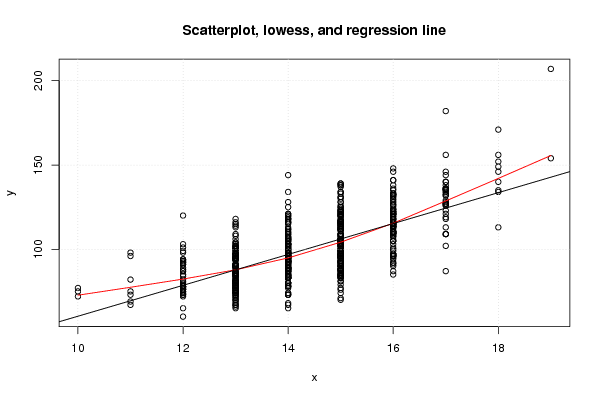
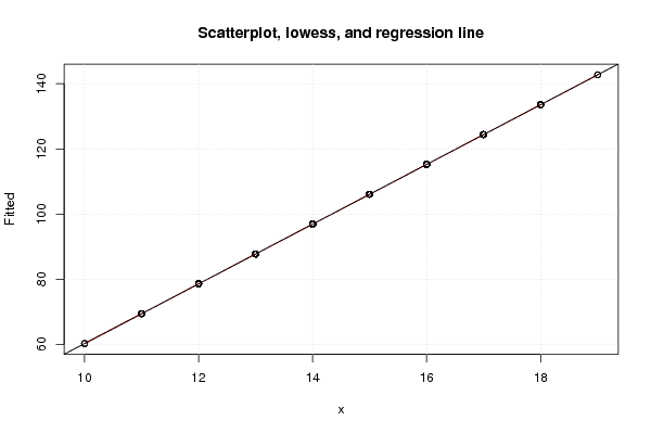
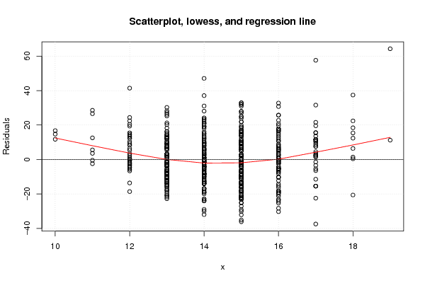
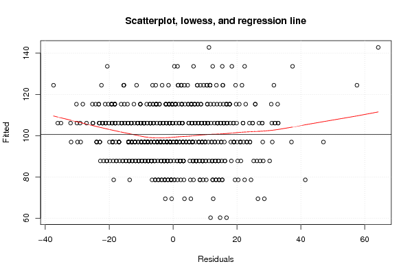
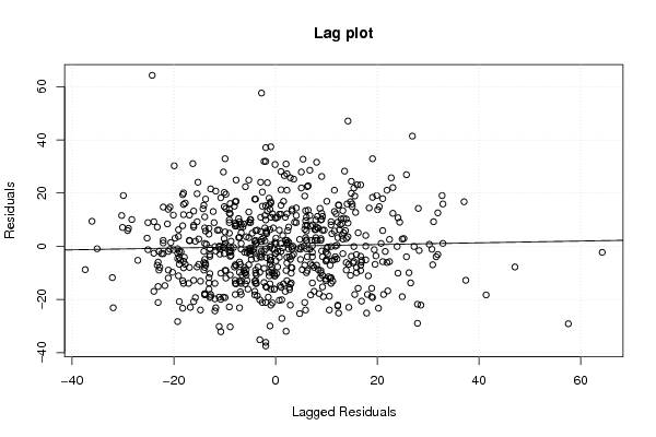
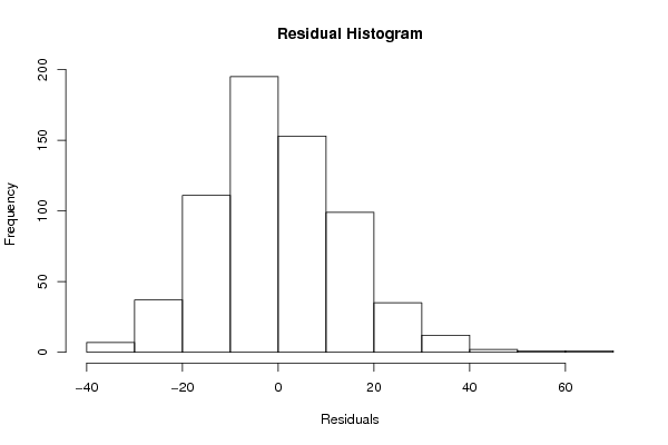
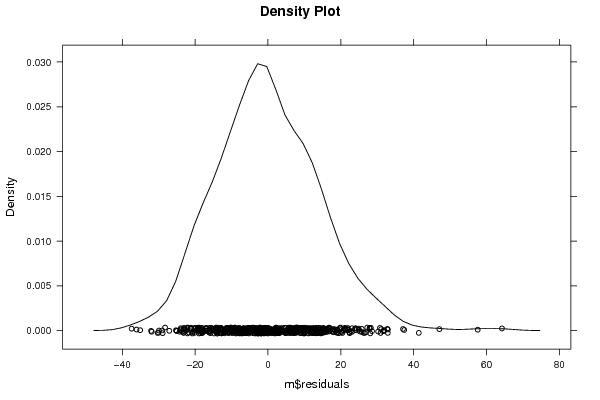
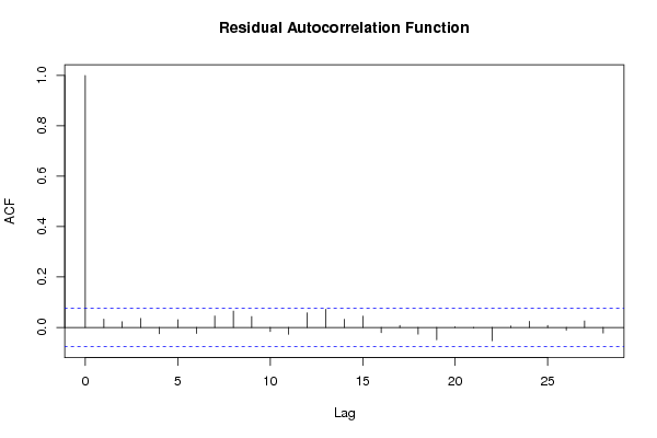
Figures (Output of Computation) | |||||||||||||||||||||||||||||||||||||||||||||||||||||||||||||
Input Parameters & R Code | |||||||||||||||||||||||||||||||||||||||||||||||||||||||||||||
| Parameters (Session): | |||||||||||||||||||||||||||||||||||||||||||||||||||||||||||||
| par1 = 0 ; | |||||||||||||||||||||||||||||||||||||||||||||||||||||||||||||
| Parameters (R input): | |||||||||||||||||||||||||||||||||||||||||||||||||||||||||||||
| par1 = 0 ; | |||||||||||||||||||||||||||||||||||||||||||||||||||||||||||||
| R code (references can be found in the software module): | |||||||||||||||||||||||||||||||||||||||||||||||||||||||||||||
par1 <- as.numeric(par1) | |||||||||||||||||||||||||||||||||||||||||||||||||||||||||||||