Repository of Reproducible Computations

Free Statistics

of Irreproducible Research!

Author's title

Author

*The author of this computation has been verified*

R Software Module

rwasp_notchedbox1.wasp

Title produced by software

Notched Boxplots

Date of computation

Sun, 13 Nov 2011 13:07:12 -0500

Cite this page as follows

Statistical Computations at FreeStatistics.org, Office for Research Development and Education, URL https://freestatistics.org/blog/index.php?v=date/2011/Nov/13/t1321207735a8upti8wp9u6yx7.htm/, Retrieved Thu, 25 Apr 2024 11:07:17 +0000

Statistical Computations at FreeStatistics.org, Office for Research Development and Education, URL https://freestatistics.org/blog/index.php?pk=141829, Retrieved Thu, 25 Apr 2024 11:07:17 +0000

QR Codes:

Paste this QR Code to cite your computation.

Original text written by user:

IsPrivate?

No (this computation is public)

User-defined keywords

Estimated Impact

Family? (F = Feedback message, R = changed R code, M = changed R Module, P = changed Parameters, D = changed Data)

-     [Aston University Statistical Software] [Morning Sickness ...] [2009-11-16 16:26:06] [74be16979710d4c4e7c6647856088456]
- R     [Aston University Statistical Software] [Morning Sickness ...] [2009-11-16 17:22:16] [74be16979710d4c4e7c6647856088456]
-   P     [T-Tests] [Morning Sickness ...] [2010-11-09 11:12:43] [3fdd735c61ad38cbc9b3393dc997cdb7]
- RM        [T-Tests] [Morning Sickness ...] [2011-11-07 09:34:35] [98fd0e87c3eb04e0cc2efde01dbafab6]
- RMP           [Notched Boxplots] [morning sickness ...] [2011-11-13 18:07:12] [ba39d87c5b07fdeb99ead4bedf199d9b] [Current]

Feedback Forum

Post a new message

Dataseries X:

Download CSV

Histogram

Boxplots

68.95	70.18
70.84	69.94
70.26	69.61
70.93	71.39
70.71	72.54
70.73	70.48
70.20	70.48
69.76	71.68
71.46	70.59
70.31	71.61
69.24	70.56
70.94	72.74
68.98	72.63
71.16	71.58
69.96	70.14
69.66	71.22
70.20	70.72
69.99	71.37
71.97	69.73
68.29	71.29
67.67	73.19
70.07	70.64
70.89	69.30
69.66	71.76
71.12	70.28
70.60	69.77
70.09	70.37
70.55	71.70
71.63	70.85
69.30	71.07

Summary of computational transaction
Raw Input	view raw input (R code)
Raw Output	view raw output of R engine
Computing time	0 seconds
R Server	'Herman Ole Andreas Wold' @ wold.wessa.net

\begin{tabular}{lllllllll}
\hline
Summary of computational transaction \tabularnewline
Raw Input & view raw input (R code)  \tabularnewline
Raw Output & view raw output of R engine  \tabularnewline
Computing time & 0 seconds \tabularnewline
R Server & 'Herman Ole Andreas Wold' @ wold.wessa.net \tabularnewline
\hline
\end{tabular}
%Source: https://freestatistics.org/blog/index.php?pk=141829&T=0

[TABLE]
[ROW][C]Summary of computational transaction[/C][/ROW]
[ROW][C]Raw Input[/C][C]view raw input (R code) [/C][/ROW]
[ROW][C]Raw Output[/C][C]view raw output of R engine [/C][/ROW]
[ROW][C]Computing time[/C][C]0 seconds[/C][/ROW]
[ROW][C]R Server[/C][C]'Herman Ole Andreas Wold' @ wold.wessa.net[/C][/ROW]
[/TABLE]
Source: https://freestatistics.org/blog/index.php?pk=141829&T=0

Globally Unique Identifier (entire table): ba.freestatistics.org/blog/index.php?pk=141829&T=0

As an alternative you can also use a QR Code:

The GUIDs for individual cells are displayed in the table below:

Summary of computational transaction
Raw Input	view raw input (R code)
Raw Output	view raw output of R engine
Computing time	0 seconds
R Server	'Herman Ole Andreas Wold' @ wold.wessa.net

Boxplot statistics
Variable	lower whisker	lower hinge	median	upper hinge	upper whisker
Drug	68.29	69.66	70.23	70.89	71.97
Placebo	69.3	70.28	70.785	71.61	73.19

\begin{tabular}{lllllllll}
\hline
Boxplot statistics \tabularnewline
Variable & lower whisker & lower hinge & median & upper hinge & upper whisker \tabularnewline
Drug & 68.29 & 69.66 & 70.23 & 70.89 & 71.97 \tabularnewline
Placebo & 69.3 & 70.28 & 70.785 & 71.61 & 73.19 \tabularnewline
\hline
\end{tabular}
%Source: https://freestatistics.org/blog/index.php?pk=141829&T=1

[TABLE]
[ROW][C]Boxplot statistics[/C][/ROW]
[ROW][C]Variable[/C][C]lower whisker[/C][C]lower hinge[/C][C]median[/C][C]upper hinge[/C][C]upper whisker[/C][/ROW]
[ROW][C]Drug[/C][C]68.29[/C][C]69.66[/C][C]70.23[/C][C]70.89[/C][C]71.97[/C][/ROW]
[ROW][C]Placebo[/C][C]69.3[/C][C]70.28[/C][C]70.785[/C][C]71.61[/C][C]73.19[/C][/ROW]
[/TABLE]
Source: https://freestatistics.org/blog/index.php?pk=141829&T=1

Globally Unique Identifier (entire table): ba.freestatistics.org/blog/index.php?pk=141829&T=1

As an alternative you can also use a QR Code:

The GUIDs for individual cells are displayed in the table below:

Boxplot statistics
Variable	lower whisker	lower hinge	median	upper hinge	upper whisker
Drug	68.29	69.66	70.23	70.89	71.97
Placebo	69.3	70.28	70.785	71.61	73.19

Boxplot Notches
Variable	lower bound	median	upper bound
Drug	69.8751853272482	70.23	70.5848146727518
Placebo	70.4013386058862	70.785	71.1686613941138

\begin{tabular}{lllllllll}
\hline
Boxplot Notches \tabularnewline
Variable & lower bound & median & upper bound \tabularnewline
Drug & 69.8751853272482 & 70.23 & 70.5848146727518 \tabularnewline
Placebo & 70.4013386058862 & 70.785 & 71.1686613941138 \tabularnewline
\hline
\end{tabular}
%Source: https://freestatistics.org/blog/index.php?pk=141829&T=2

[TABLE]
[ROW][C]Boxplot Notches[/C][/ROW]
[ROW][C]Variable[/C][C]lower bound[/C][C]median[/C][C]upper bound[/C][/ROW]
[ROW][C]Drug[/C][C]69.8751853272482[/C][C]70.23[/C][C]70.5848146727518[/C][/ROW]
[ROW][C]Placebo[/C][C]70.4013386058862[/C][C]70.785[/C][C]71.1686613941138[/C][/ROW]
[/TABLE]
Source: https://freestatistics.org/blog/index.php?pk=141829&T=2

Globally Unique Identifier (entire table): ba.freestatistics.org/blog/index.php?pk=141829&T=2

As an alternative you can also use a QR Code:

The GUIDs for individual cells are displayed in the table below:

Boxplot Notches
Variable	lower bound	median	upper bound
Drug	69.8751853272482	70.23	70.5848146727518
Placebo	70.4013386058862	70.785	71.1686613941138

Figure 1

PNG link

Postscript link

PDF link

Parameters (Session):

par1 = yellow ;

Parameters (R input):

par1 = yellow ;

R code (references can be found in the software module):

z <- as.data.frame(t(y))
bitmap(file='test1.png')
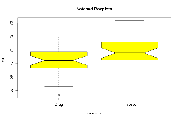
(r<-boxplot(z ,xlab=xlab,ylab=ylab,main=main,notch=TRUE,col=par1))
dev.off()
load(file='createtable')
a<-table.start()
a<-table.row.start(a)
a<-table.element(a,hyperlink('overview.htm','Boxplot statistics','Boxplot overview'),6,TRUE)
a<-table.row.end(a)
a<-table.row.start(a)
a<-table.element(a,'Variable',1,TRUE)
a<-table.element(a,hyperlink('lower_whisker.htm','lower whisker','definition of lower whisker'),1,TRUE)
a<-table.element(a,hyperlink('lower_hinge.htm','lower hinge','definition of lower hinge'),1,TRUE)
a<-table.element(a,hyperlink('central_tendency.htm','median','definitions about measures of central tendency'),1,TRUE)
a<-table.element(a,hyperlink('upper_hinge.htm','upper hinge','definition of upper hinge'),1,TRUE)
a<-table.element(a,hyperlink('upper_whisker.htm','upper whisker','definition of upper whisker'),1,TRUE)
a<-table.row.end(a)
for (i in 1:length(y[,1]))
{
a<-table.row.start(a)
a<-table.element(a,dimnames(t(x))[[2]][i],1,TRUE)
for (j in 1:5)
{
a<-table.element(a,r$stats[j,i])
}
a<-table.row.end(a)
}
a<-table.end(a)
table.save(a,file='mytable.tab')
a<-table.start()
a<-table.row.start(a)
a<-table.element(a,'Boxplot Notches',4,TRUE)
a<-table.row.end(a)
a<-table.row.start(a)
a<-table.element(a,'Variable',1,TRUE)
a<-table.element(a,'lower bound',1,TRUE)
a<-table.element(a,'median',1,TRUE)
a<-table.element(a,'upper bound',1,TRUE)
a<-table.row.end(a)
for (i in 1:length(y[,1]))
{
a<-table.row.start(a)
a<-table.element(a,dimnames(t(x))[[2]][i],1,TRUE)
a<-table.element(a,r$conf[1,i])
a<-table.element(a,r$stats[3,i])
a<-table.element(a,r$conf[2,i])
a<-table.row.end(a)
}
a<-table.end(a)
table.save(a,file='mytable1.tab')

Free Statistics

Description of Statistical Computation

Tree of Dependent Computations

Dataset

Tables (Output of Computation)

Figures (Output of Computation)

Input Parameters & R Code