Free Statistics

of Irreproducible Research!

Author's title

Author*The author of this computation has been verified*
R Software Module--
Title produced by softwarePaired and Unpaired Two Samples Tests about the Mean
Date of computationSun, 13 Nov 2011 12:26:18 -0500
Cite this page as followsStatistical Computations at FreeStatistics.org, Office for Research Development and Education, URL https://freestatistics.org/blog/index.php?v=date/2011/Nov/13/t13212051863dnksudr9rrid4y.htm/, Retrieved Tue, 16 Apr 2024 18:05:46 +0000
Statistical Computations at FreeStatistics.org, Office for Research Development and Education, URL https://freestatistics.org/blog/index.php?pk=141816, Retrieved Tue, 16 Apr 2024 18:05:46 +0000
QR Codes:

Original text written by user:
IsPrivate?No (this computation is public)
User-defined keywords
Estimated Impact87
Family? (F = Feedback message, R = changed R code, M = changed R Module, P = changed Parameters, D = changed Data)
-     [Paired and Unpaired Two Samples Tests about the Mean] [] [2010-11-16 19:06:11] [f3d662049ef6875ba0c96bb458434b66]
- RM      [Paired and Unpaired Two Samples Tests about the Mean] [] [2011-11-13 17:26:18] [583fc5a74bfa894f261a865501f20e1c] [Current]
Feedback Forum

Post a new message
Dataseries X:
1280	1024
1024	768
1120	700
1024	768
1280	800
1280	1024
1280	800
1024	768
1280	800
1280	1024
1280	800
1280	800
1280	1024
1688	949
1440	900
1600	1200
1280	800
1280	800
1280	768
1176	735
1280	800
1503	845
1440	900
1366	768
1280	768
1024	768
1280	800
2560	1440
1280	768
1024	768
1280	1024
1280	800
1440	900
1280	800
1440	900
1024	768
1440	900
1143	857
1280	800
1440	900
1280	800
1366	768
1024	768
1408	880
1366	768
1176	735
1920	1200
1257	785
1280	800
1280	800
1440	900
1680	1050
1440	900
1024	768
1140	641
1280	1024
1280	800
1280	800
1280	800
1280	800
1440	900
1280	800
1152	864
1280	1024
1280	800
1440	900
1280	800
1280	1024
1440	900
1280	800
1280	800
1440	900
1280	800
1280	1024
1600	900
1024	768
1366	768
1280	800
1280	800
1440	900
1366	768
1280	800
1024	768
1280	800
1440	900
1280	800
1280	800
1408	880
1280	800
1600	900
1600	900
1680	1050
1440	900
1440	900
917	550
1280	800
1760	990
1280	800
1280	800
1280	800
1024	768
1366	768
1440	900
1280	800
1280	1024
1920	1080
1024	768
1024	768
1600	900
1117	698
1440	900
983	737
1024	768
1024	640
1280	800
1440	900
1280	800
1280	800
1280	800
1440	900
1280	800
1024	768
1024	768
1152	864
1280	768
1024	768
1366	768
1680	1050
1680	1050
1280	800
1366	768
1024	768
1440	900
1024	768
1280	800
1280	800
1280	800
1024	768
1280	800


Summary of computational transaction
Raw Inputview raw input (R code)
Raw Outputview raw output of R engine
Computing time2 seconds
R Server'AstonUniversity' @ aston.wessa.net

\begin{tabular}{lllllllll}
\hline
Summary of computational transaction \tabularnewline
Raw Input & view raw input (R code)  \tabularnewline
Raw Output & view raw output of R engine  \tabularnewline
Computing time & 2 seconds \tabularnewline
R Server & 'AstonUniversity' @ aston.wessa.net \tabularnewline
\hline
\end{tabular}
%Source: https://freestatistics.org/blog/index.php?pk=141816&T=0

[TABLE]
[ROW][C]Summary of computational transaction[/C][/ROW]
[ROW][C]Raw Input[/C][C]view raw input (R code) [/C][/ROW]
[ROW][C]Raw Output[/C][C]view raw output of R engine [/C][/ROW]
[ROW][C]Computing time[/C][C]2 seconds[/C][/ROW]
[ROW][C]R Server[/C][C]'AstonUniversity' @ aston.wessa.net[/C][/ROW]
[/TABLE]
Source: https://freestatistics.org/blog/index.php?pk=141816&T=0

Globally Unique Identifier (entire table): ba.freestatistics.org/blog/index.php?pk=141816&T=0

As an alternative you can also use a QR Code:  

The GUIDs for individual cells are displayed in the table below:

Summary of computational transaction
Raw Inputview raw input (R code)
Raw Outputview raw output of R engine
Computing time2 seconds
R Server'AstonUniversity' @ aston.wessa.net


Two Sample t-test (paired)
Difference: Mean1 - Mean2464.647482014389
t-stat37.5522043961123
df138
p-value2.54326870522062e-74
H0 value0
Alternativetwo.sided
CI Level0.95
CI[440.181565119337,489.11339890944]
F-test to compare two variances
F-stat3.50863251862628
df138
p-value9.49684775264359e-13
H0 value1
Alternativetwo.sided
CI Level0.95
CI[2.50968562553,4.90519690017432]

\begin{tabular}{lllllllll}
\hline
Two Sample t-test (paired) \tabularnewline
Difference: Mean1 - Mean2 & 464.647482014389 \tabularnewline
t-stat & 37.5522043961123 \tabularnewline
df & 138 \tabularnewline
p-value & 2.54326870522062e-74 \tabularnewline
H0 value & 0 \tabularnewline
Alternative & two.sided \tabularnewline
CI Level & 0.95 \tabularnewline
CI & [440.181565119337,489.11339890944] \tabularnewline
F-test to compare two variances \tabularnewline
F-stat & 3.50863251862628 \tabularnewline
df & 138 \tabularnewline
p-value & 9.49684775264359e-13 \tabularnewline
H0 value & 1 \tabularnewline
Alternative & two.sided \tabularnewline
CI Level & 0.95 \tabularnewline
CI & [2.50968562553,4.90519690017432] \tabularnewline
\hline
\end{tabular}
%Source: https://freestatistics.org/blog/index.php?pk=141816&T=1

[TABLE]
[ROW][C]Two Sample t-test (paired)[/C][/ROW]
[ROW][C]Difference: Mean1 - Mean2[/C][C]464.647482014389[/C][/ROW]
[ROW][C]t-stat[/C][C]37.5522043961123[/C][/ROW]
[ROW][C]df[/C][C]138[/C][/ROW]
[ROW][C]p-value[/C][C]2.54326870522062e-74[/C][/ROW]
[ROW][C]H0 value[/C][C]0[/C][/ROW]
[ROW][C]Alternative[/C][C]two.sided[/C][/ROW]
[ROW][C]CI Level[/C][C]0.95[/C][/ROW]
[ROW][C]CI[/C][C][440.181565119337,489.11339890944][/C][/ROW]
[ROW][C]F-test to compare two variances[/C][/ROW]
[ROW][C]F-stat[/C][C]3.50863251862628[/C][/ROW]
[ROW][C]df[/C][C]138[/C][/ROW]
[ROW][C]p-value[/C][C]9.49684775264359e-13[/C][/ROW]
[ROW][C]H0 value[/C][C]1[/C][/ROW]
[ROW][C]Alternative[/C][C]two.sided[/C][/ROW]
[ROW][C]CI Level[/C][C]0.95[/C][/ROW]
[ROW][C]CI[/C][C][2.50968562553,4.90519690017432][/C][/ROW]
[/TABLE]
Source: https://freestatistics.org/blog/index.php?pk=141816&T=1

Globally Unique Identifier (entire table): ba.freestatistics.org/blog/index.php?pk=141816&T=1

As an alternative you can also use a QR Code:  

The GUIDs for individual cells are displayed in the table below:

Two Sample t-test (paired)
Difference: Mean1 - Mean2464.647482014389
t-stat37.5522043961123
df138
p-value2.54326870522062e-74
H0 value0
Alternativetwo.sided
CI Level0.95
CI[440.181565119337,489.11339890944]
F-test to compare two variances
F-stat3.50863251862628
df138
p-value9.49684775264359e-13
H0 value1
Alternativetwo.sided
CI Level0.95
CI[2.50968562553,4.90519690017432]


Welch Two Sample t-test (paired)
Difference: Mean1 - Mean2464.647482014389
t-stat37.5522043961123
df138
p-value2.54326870522062e-74
H0 value0
Alternativetwo.sided
CI Level0.95
CI[440.181565119337,489.11339890944]

\begin{tabular}{lllllllll}
\hline
Welch Two Sample t-test (paired) \tabularnewline
Difference: Mean1 - Mean2 & 464.647482014389 \tabularnewline
t-stat & 37.5522043961123 \tabularnewline
df & 138 \tabularnewline
p-value & 2.54326870522062e-74 \tabularnewline
H0 value & 0 \tabularnewline
Alternative & two.sided \tabularnewline
CI Level & 0.95 \tabularnewline
CI & [440.181565119337,489.11339890944] \tabularnewline
\hline
\end{tabular}
%Source: https://freestatistics.org/blog/index.php?pk=141816&T=2

[TABLE]
[ROW][C]Welch Two Sample t-test (paired)[/C][/ROW]
[ROW][C]Difference: Mean1 - Mean2[/C][C]464.647482014389[/C][/ROW]
[ROW][C]t-stat[/C][C]37.5522043961123[/C][/ROW]
[ROW][C]df[/C][C]138[/C][/ROW]
[ROW][C]p-value[/C][C]2.54326870522062e-74[/C][/ROW]
[ROW][C]H0 value[/C][C]0[/C][/ROW]
[ROW][C]Alternative[/C][C]two.sided[/C][/ROW]
[ROW][C]CI Level[/C][C]0.95[/C][/ROW]
[ROW][C]CI[/C][C][440.181565119337,489.11339890944][/C][/ROW]
[/TABLE]
Source: https://freestatistics.org/blog/index.php?pk=141816&T=2

Globally Unique Identifier (entire table): ba.freestatistics.org/blog/index.php?pk=141816&T=2

As an alternative you can also use a QR Code:  

The GUIDs for individual cells are displayed in the table below:

Welch Two Sample t-test (paired)
Difference: Mean1 - Mean2464.647482014389
t-stat37.5522043961123
df138
p-value2.54326870522062e-74
H0 value0
Alternativetwo.sided
CI Level0.95
CI[440.181565119337,489.11339890944]


Wicoxon rank sum test with continuity correction (paired)
W9730
p-value7.46639785555896e-25
H0 value0
Alternativetwo.sided
Kolmogorov-Smirnov Test to compare Distributions of two Samples
KS Statistic0.856115107913669
p-value0
Kolmogorov-Smirnov Test to compare Distributional Shape of two Samples
KS Statistic0.402877697841727
p-value3.18307269431273e-10

\begin{tabular}{lllllllll}
\hline
Wicoxon rank sum test with continuity correction (paired) \tabularnewline
W & 9730 \tabularnewline
p-value & 7.46639785555896e-25 \tabularnewline
H0 value & 0 \tabularnewline
Alternative & two.sided \tabularnewline
Kolmogorov-Smirnov Test to compare Distributions of two Samples \tabularnewline
KS Statistic & 0.856115107913669 \tabularnewline
p-value & 0 \tabularnewline
Kolmogorov-Smirnov Test to compare Distributional Shape of two Samples \tabularnewline
KS Statistic & 0.402877697841727 \tabularnewline
p-value & 3.18307269431273e-10 \tabularnewline
\hline
\end{tabular}
%Source: https://freestatistics.org/blog/index.php?pk=141816&T=3

[TABLE]
[ROW][C]Wicoxon rank sum test with continuity correction (paired)[/C][/ROW]
[ROW][C]W[/C][C]9730[/C][/ROW]
[ROW][C]p-value[/C][C]7.46639785555896e-25[/C][/ROW]
[ROW][C]H0 value[/C][C]0[/C][/ROW]
[ROW][C]Alternative[/C][C]two.sided[/C][/ROW]
[ROW][C]Kolmogorov-Smirnov Test to compare Distributions of two Samples[/C][/ROW]
[ROW][C]KS Statistic[/C][C]0.856115107913669[/C][/ROW]
[ROW][C]p-value[/C][C]0[/C][/ROW]
[ROW][C]Kolmogorov-Smirnov Test to compare Distributional Shape of two Samples[/C][/ROW]
[ROW][C]KS Statistic[/C][C]0.402877697841727[/C][/ROW]
[ROW][C]p-value[/C][C]3.18307269431273e-10[/C][/ROW]
[/TABLE]
Source: https://freestatistics.org/blog/index.php?pk=141816&T=3

Globally Unique Identifier (entire table): ba.freestatistics.org/blog/index.php?pk=141816&T=3

As an alternative you can also use a QR Code:  

The GUIDs for individual cells are displayed in the table below:

Wicoxon rank sum test with continuity correction (paired)
W9730
p-value7.46639785555896e-25
H0 value0
Alternativetwo.sided
Kolmogorov-Smirnov Test to compare Distributions of two Samples
KS Statistic0.856115107913669
p-value0
Kolmogorov-Smirnov Test to compare Distributional Shape of two Samples
KS Statistic0.402877697841727
p-value3.18307269431273e-10


Parameters (Session):
par1 = 1 ; par2 = 2 ; par3 = 0.95 ; par4 = two.sided ; par5 = paired ; par6 = 0 ;
Parameters (R input):
par1 = 1 ; par2 = 2 ; par3 = 0.95 ; par4 = two.sided ; par5 = paired ; par6 = 0 ; par7 = ; par8 = ; par9 = ; par10 = ; par11 = ; par12 = ; par13 = ; par14 = ; par15 = ; par16 = ; par17 = ; par18 = ; par19 = ; par20 = ;
R code (references can be found in the software module):
par1 <- as.numeric(par1) #column number of first sample
par2 <- as.numeric(par2) #column number of second sample
par3 <- as.numeric(par3) #confidence (= 1 - alpha)
if (par5 == 'unpaired') paired <- FALSE else paired <- TRUE
par6 <- as.numeric(par6) #H0
z <- t(y)
if (par1 == par2) stop('Please, select two different column numbers')
if (par1 < 1) stop('Please, select a column number greater than zero for the first sample')
if (par2 < 1) stop('Please, select a column number greater than zero for the second sample')
if (par1 > length(z[1,])) stop('The column number for the first sample should be smaller')
if (par2 > length(z[1,])) stop('The column number for the second sample should be smaller')
if (par3 <= 0) stop('The confidence level should be larger than zero')
if (par3 >= 1) stop('The confidence level should be smaller than zero')
(r.t <- t.test(z[,par1],z[,par2],var.equal=TRUE,alternative=par4,paired=paired,mu=par6,conf.level=par3))
(v.t <- var.test(z[,par1],z[,par2],conf.level=par3))
(r.w <- t.test(z[,par1],z[,par2],var.equal=FALSE,alternative=par4,paired=paired,mu=par6,conf.level=par3))
(w.t <- wilcox.test(z[,par1],z[,par2],alternative=par4,paired=paired,mu=par6,conf.level=par3))
(ks.t <- ks.test(z[,par1],z[,par2],alternative=par4))
m1 <- mean(z[,par1],na.rm=T)
m2 <- mean(z[,par2],na.rm=T)
mdiff <- m1 - m2
newsam1 <- z[!is.na(z[,par1]),par1]
newsam2 <- z[,par2]+mdiff
newsam2 <- newsam2[!is.na(newsam2)]
(ks1.t <- ks.test(newsam1,newsam2,alternative=par4))
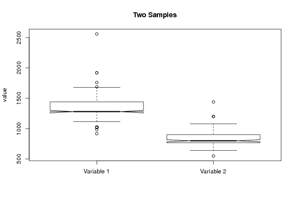
mydf <- data.frame(cbind(z[,par1],z[,par2]))
colnames(mydf) <- c('Variable 1','Variable 2')
bitmap(file='test1.png')
boxplot(mydf, notch=TRUE, ylab='value',main=main)
dev.off()
bitmap(file='test2.png')
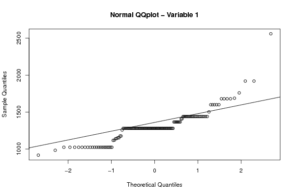
qqnorm(z[,par1],main='Normal QQplot - Variable 1')
qqline(z[,par1])
dev.off()
bitmap(file='test3.png')
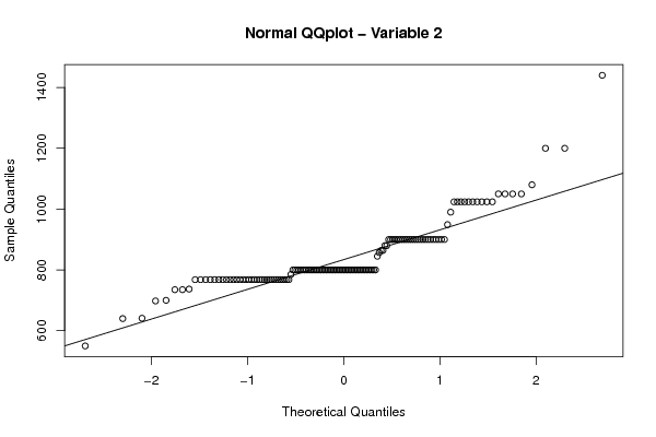
qqnorm(z[,par2],main='Normal QQplot - Variable 2')
qqline(z[,par2])
dev.off()
load(file='createtable')
a<-table.start()
a<-table.row.start(a)
a<-table.element(a,paste('Two Sample t-test (',par5,')',sep=''),2,TRUE)
a<-table.row.end(a)
if(!paired){
a<-table.row.start(a)
a<-table.element(a,'Mean of Sample 1',header=TRUE)
a<-table.element(a,r.t$estimate[[1]])
a<-table.row.end(a)
a<-table.row.start(a)
a<-table.element(a,'Mean of Sample 2',header=TRUE)
a<-table.element(a,r.t$estimate[[2]])
a<-table.row.end(a)
} else {
a<-table.row.start(a)
a<-table.element(a,'Difference: Mean1 - Mean2',header=TRUE)
a<-table.element(a,r.t$estimate)
a<-table.row.end(a)
}
a<-table.row.start(a)
a<-table.element(a,'t-stat',header=TRUE)
a<-table.element(a,r.t$statistic[[1]])
a<-table.row.end(a)
a<-table.row.start(a)
a<-table.element(a,'df',header=TRUE)
a<-table.element(a,r.t$parameter[[1]])
a<-table.row.end(a)
a<-table.row.start(a)
a<-table.element(a,'p-value',header=TRUE)
a<-table.element(a,r.t$p.value)
a<-table.row.end(a)
a<-table.row.start(a)
a<-table.element(a,'H0 value',header=TRUE)
a<-table.element(a,r.t$null.value[[1]])
a<-table.row.end(a)
a<-table.row.start(a)
a<-table.element(a,'Alternative',header=TRUE)
a<-table.element(a,r.t$alternative)
a<-table.row.end(a)
a<-table.row.start(a)
a<-table.element(a,'CI Level',header=TRUE)
a<-table.element(a,attr(r.t$conf.int,'conf.level'))
a<-table.row.end(a)
a<-table.row.start(a)
a<-table.element(a,'CI',header=TRUE)
a<-table.element(a,paste('[',r.t$conf.int[1],',',r.t$conf.int[2],']',sep=''))
a<-table.row.end(a)
a<-table.row.start(a)
a<-table.element(a,'F-test to compare two variances',2,TRUE)
a<-table.row.end(a)
a<-table.row.start(a)
a<-table.element(a,'F-stat',header=TRUE)
a<-table.element(a,v.t$statistic[[1]])
a<-table.row.end(a)
a<-table.row.start(a)
a<-table.element(a,'df',header=TRUE)
a<-table.element(a,v.t$parameter[[1]])
a<-table.row.end(a)
a<-table.row.start(a)
a<-table.element(a,'p-value',header=TRUE)
a<-table.element(a,v.t$p.value)
a<-table.row.end(a)
a<-table.row.start(a)
a<-table.element(a,'H0 value',header=TRUE)
a<-table.element(a,v.t$null.value[[1]])
a<-table.row.end(a)
a<-table.row.start(a)
a<-table.element(a,'Alternative',header=TRUE)
a<-table.element(a,v.t$alternative)
a<-table.row.end(a)
a<-table.row.start(a)
a<-table.element(a,'CI Level',header=TRUE)
a<-table.element(a,attr(v.t$conf.int,'conf.level'))
a<-table.row.end(a)
a<-table.row.start(a)
a<-table.element(a,'CI',header=TRUE)
a<-table.element(a,paste('[',v.t$conf.int[1],',',v.t$conf.int[2],']',sep=''))
a<-table.row.end(a)
a<-table.end(a)
table.save(a,file='mytable.tab')
a<-table.start()
a<-table.row.start(a)
a<-table.element(a,paste('Welch Two Sample t-test (',par5,')',sep=''),2,TRUE)
a<-table.row.end(a)
if(!paired){
a<-table.row.start(a)
a<-table.element(a,'Mean of Sample 1',header=TRUE)
a<-table.element(a,r.w$estimate[[1]])
a<-table.row.end(a)
a<-table.row.start(a)
a<-table.element(a,'Mean of Sample 2',header=TRUE)
a<-table.element(a,r.w$estimate[[2]])
a<-table.row.end(a)
} else {
a<-table.row.start(a)
a<-table.element(a,'Difference: Mean1 - Mean2',header=TRUE)
a<-table.element(a,r.w$estimate)
a<-table.row.end(a)
}
a<-table.row.start(a)
a<-table.element(a,'t-stat',header=TRUE)
a<-table.element(a,r.w$statistic[[1]])
a<-table.row.end(a)
a<-table.row.start(a)
a<-table.element(a,'df',header=TRUE)
a<-table.element(a,r.w$parameter[[1]])
a<-table.row.end(a)
a<-table.row.start(a)
a<-table.element(a,'p-value',header=TRUE)
a<-table.element(a,r.w$p.value)
a<-table.row.end(a)
a<-table.row.start(a)
a<-table.element(a,'H0 value',header=TRUE)
a<-table.element(a,r.w$null.value[[1]])
a<-table.row.end(a)
a<-table.row.start(a)
a<-table.element(a,'Alternative',header=TRUE)
a<-table.element(a,r.w$alternative)
a<-table.row.end(a)
a<-table.row.start(a)
a<-table.element(a,'CI Level',header=TRUE)
a<-table.element(a,attr(r.w$conf.int,'conf.level'))
a<-table.row.end(a)
a<-table.row.start(a)
a<-table.element(a,'CI',header=TRUE)
a<-table.element(a,paste('[',r.w$conf.int[1],',',r.w$conf.int[2],']',sep=''))
a<-table.row.end(a)
a<-table.end(a)
table.save(a,file='mytable1.tab')
a<-table.start()
a<-table.row.start(a)
a<-table.element(a,paste('Wicoxon rank sum test with continuity correction (',par5,')',sep=''),2,TRUE)
a<-table.row.end(a)
a<-table.row.start(a)
a<-table.element(a,'W',header=TRUE)
a<-table.element(a,w.t$statistic[[1]])
a<-table.row.end(a)
a<-table.row.start(a)
a<-table.element(a,'p-value',header=TRUE)
a<-table.element(a,w.t$p.value)
a<-table.row.end(a)
a<-table.row.start(a)
a<-table.element(a,'H0 value',header=TRUE)
a<-table.element(a,w.t$null.value[[1]])
a<-table.row.end(a)
a<-table.row.start(a)
a<-table.element(a,'Alternative',header=TRUE)
a<-table.element(a,w.t$alternative)
a<-table.row.end(a)
a<-table.row.start(a)
a<-table.element(a,'Kolmogorov-Smirnov Test to compare Distributions of two Samples',2,TRUE)
a<-table.row.end(a)
a<-table.row.start(a)
a<-table.element(a,'KS Statistic',header=TRUE)
a<-table.element(a,ks.t$statistic[[1]])
a<-table.row.end(a)
a<-table.row.start(a)
a<-table.element(a,'p-value',header=TRUE)
a<-table.element(a,ks.t$p.value)
a<-table.row.end(a)
a<-table.row.start(a)
a<-table.element(a,'Kolmogorov-Smirnov Test to compare Distributional Shape of two Samples',2,TRUE)
a<-table.row.end(a)
a<-table.row.start(a)
a<-table.element(a,'KS Statistic',header=TRUE)
a<-table.element(a,ks1.t$statistic[[1]])
a<-table.row.end(a)
a<-table.row.start(a)
a<-table.element(a,'p-value',header=TRUE)
a<-table.element(a,ks1.t$p.value)
a<-table.row.end(a)
a<-table.end(a)
table.save(a,file='mytable2.tab')