Free Statistics
of Irreproducible Research!
Description of Statistical Computation | ||||||||||||||||||||||||||||||
|---|---|---|---|---|---|---|---|---|---|---|---|---|---|---|---|---|---|---|---|---|---|---|---|---|---|---|---|---|---|---|
| Author's title | ||||||||||||||||||||||||||||||
| Author | *The author of this computation has been verified* | |||||||||||||||||||||||||||||
| R Software Module | rwasp_Distributional Plots.wasp | |||||||||||||||||||||||||||||
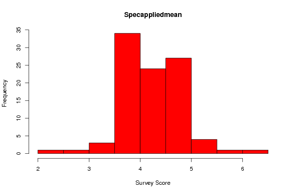
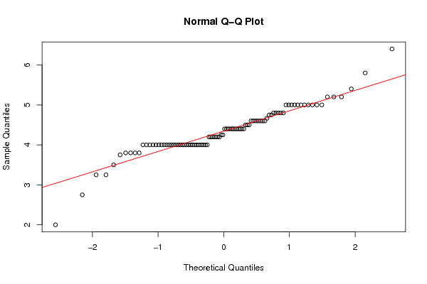
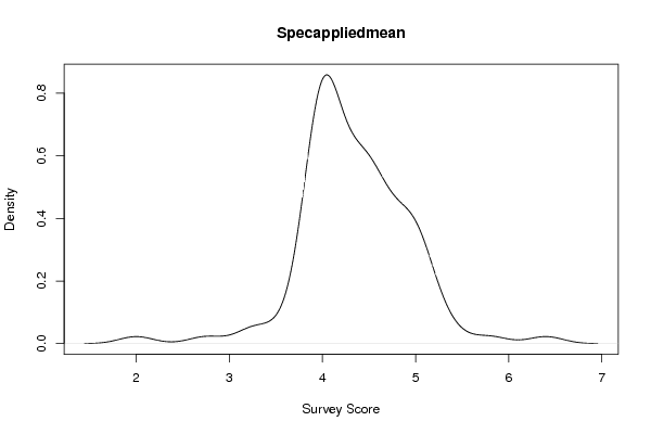
| Title produced by software | Histogram, QQplot and Density | |||||||||||||||||||||||||||||
| Date of computation | Mon, 07 Nov 2011 18:17:34 -0500 | |||||||||||||||||||||||||||||
| Cite this page as follows | Statistical Computations at FreeStatistics.org, Office for Research Development and Education, URL https://freestatistics.org/blog/index.php?v=date/2011/Nov/07/t1320707868stgclscw2dhtkm2.htm/, Retrieved Thu, 25 Apr 2024 22:28:54 +0000 | |||||||||||||||||||||||||||||
| Statistical Computations at FreeStatistics.org, Office for Research Development and Education, URL https://freestatistics.org/blog/index.php?pk=140465, Retrieved Thu, 25 Apr 2024 22:28:54 +0000 | ||||||||||||||||||||||||||||||
| QR Codes: | ||||||||||||||||||||||||||||||
|
| ||||||||||||||||||||||||||||||
| Original text written by user: | ||||||||||||||||||||||||||||||
| IsPrivate? | No (this computation is public) | |||||||||||||||||||||||||||||
| User-defined keywords | ||||||||||||||||||||||||||||||
| Estimated Impact | 140 | |||||||||||||||||||||||||||||
Tree of Dependent Computations | ||||||||||||||||||||||||||||||
| Family? (F = Feedback message, R = changed R code, M = changed R Module, P = changed Parameters, D = changed Data) | ||||||||||||||||||||||||||||||
| - [Histogram, QQplot and Density] [Week 4 Comp 3] [2011-10-30 08:43:48] [f30aa6c31987f6fcaa8cd16e7d6e8a58] - R D [Histogram, QQplot and Density] [Histogram and QQ ...] [2011-11-07 23:14:47] [553711af6a3a99aac240956ee7ba8417] - D [Histogram, QQplot and Density] [Histogram and QQ ...] [2011-11-07 23:16:29] [553711af6a3a99aac240956ee7ba8417] - D [Histogram, QQplot and Density] [Histogram and QQ ...] [2011-11-07 23:17:34] [50ef738b441df67da458e2632ba394c1] [Current] | ||||||||||||||||||||||||||||||
| Feedback Forum | ||||||||||||||||||||||||||||||
Post a new message | ||||||||||||||||||||||||||||||
Dataset | ||||||||||||||||||||||||||||||
| Dataseries X: | ||||||||||||||||||||||||||||||
4.6 4 4.8 4 5 5 4 4 4.4 4 4 5 3.8 4.6 4 4.6 4.666666667 4 4 4.4 4.8 5.8 4.6 4.75 5 2.75 4 3.8 4.4 4.8 4.25 4.4 4 4.5 5 3.5 2 4.4 4.4 4.25 3.25 4.2 4.75 4.4 4 4.2 5 4.6 4.4 4 4.4 4.5 5.2 4.4 3.25 4.6 3.75 5 3.8 4 5.4 5 5 4.2 4.4 4 4.6 4.2 5.2 6.4 4 4 5 4 4.2 4 4 4 4 4 4.2 4 4 4 5.2 4.2 4.8 4 4.8 5 4.6 4 4.4 4 3.8 4.5 | ||||||||||||||||||||||||||||||
Tables (Output of Computation) | ||||||||||||||||||||||||||||||
| ||||||||||||||||||||||||||||||
Figures (Output of Computation) | ||||||||||||||||||||||||||||||
Input Parameters & R Code | ||||||||||||||||||||||||||||||
| Parameters (Session): | ||||||||||||||||||||||||||||||
| par1 = 15 ; | ||||||||||||||||||||||||||||||
| Parameters (R input): | ||||||||||||||||||||||||||||||
| par1 = 15 ; | ||||||||||||||||||||||||||||||
| R code (references can be found in the software module): | ||||||||||||||||||||||||||||||
bitmap(file='test1.png') | ||||||||||||||||||||||||||||||