Repository of Reproducible Computations

Free Statistics

of Irreproducible Research!

Author's title

Author

*The author of this computation has been verified*

R Software Module

rwasp_arimaforecasting.wasp

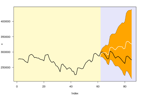
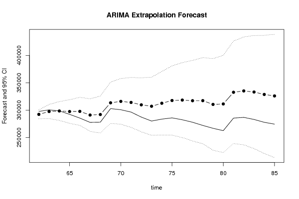
Title produced by software

ARIMA Forecasting

Date of computation

Fri, 23 Dec 2011 14:41:16 -0500

Cite this page as follows

Statistical Computations at FreeStatistics.org, Office for Research Development and Education, URL https://freestatistics.org/blog/index.php?v=date/2011/Dec/23/t1324669305e00p9pa2tvlc3x8.htm/, Retrieved Mon, 29 Apr 2024 22:37:20 +0000

Statistical Computations at FreeStatistics.org, Office for Research Development and Education, URL https://freestatistics.org/blog/index.php?pk=160684, Retrieved Mon, 29 Apr 2024 22:37:20 +0000

QR Codes:

Paste this QR Code to cite your computation.

Original text written by user:

IsPrivate?

No (this computation is public)

User-defined keywords

Estimated Impact

117

Family? (F = Feedback message, R = changed R code, M = changed R Module, P = changed Parameters, D = changed Data)

-     [Univariate Explorative Data Analysis] [Run Sequence gebo...] [2008-12-12 13:32:37] [76963dc1903f0f612b6153510a3818cf]
- R  D  [Univariate Explorative Data Analysis] [Run Sequence gebo...] [2008-12-17 12:14:40] [76963dc1903f0f612b6153510a3818cf]
-         [Univariate Explorative Data Analysis] [Run Sequence Plot...] [2008-12-22 18:19:51] [1ce0d16c8f4225c977b42c8fa93bc163]
- RMP       [(Partial) Autocorrelation Function] [Identifying Integ...] [2009-11-22 12:16:10] [b98453cac15ba1066b407e146608df68]
-    D        [(Partial) Autocorrelation Function] [ACF van Y(t) (d=0...] [2009-11-26 00:58:58] [9717cb857c153ca3061376906953b329]
-   P           [(Partial) Autocorrelation Function] [ACF van Y(t) (d=1...] [2009-11-26 17:32:24] [9717cb857c153ca3061376906953b329]
-   P             [(Partial) Autocorrelation Function] [ACF van Y(t) (d=1...] [2009-11-26 17:41:56] [9717cb857c153ca3061376906953b329]
- RMP               [ARIMA Backward Selection] [ARIMA Backward Se...] [2009-12-03 01:42:16] [9717cb857c153ca3061376906953b329]
-                     [ARIMA Backward Selection] [Paper Arima backw...] [2011-12-20 17:11:29] [abc1cbe561c2c4615f632bb3153b1275]
- RMP                   [ARIMA Forecasting] [Paper Arima forec...] [2011-12-22 18:40:24] [abc1cbe561c2c4615f632bb3153b1275]
- R PD                      [ARIMA Forecasting] [Arima Forecasting...] [2011-12-23 19:41:16] [8aedcf735e397266388b06f47fe45218] [Current]

Feedback Forum

Post a new message

Dataseries X:

Download CSV

Histogram

Boxplots

Summary of computational transaction
Raw Input	view raw input (R code)
Raw Output	view raw output of R engine
Computing time	1 seconds
R Server	'Herman Ole Andreas Wold' @ wold.wessa.net

\begin{tabular}{lllllllll}
\hline
Summary of computational transaction \tabularnewline
Raw Input & view raw input (R code)  \tabularnewline
Raw Output & view raw output of R engine  \tabularnewline
Computing time & 1 seconds \tabularnewline
R Server & 'Herman Ole Andreas Wold' @ wold.wessa.net \tabularnewline
\hline
\end{tabular}
%Source: https://freestatistics.org/blog/index.php?pk=160684&T=0

[TABLE]
[ROW][C]Summary of computational transaction[/C][/ROW]
[ROW][C]Raw Input[/C][C]view raw input (R code) [/C][/ROW]
[ROW][C]Raw Output[/C][C]view raw output of R engine [/C][/ROW]
[ROW][C]Computing time[/C][C]1 seconds[/C][/ROW]
[ROW][C]R Server[/C][C]'Herman Ole Andreas Wold' @ wold.wessa.net[/C][/ROW]
[/TABLE]
Source: https://freestatistics.org/blog/index.php?pk=160684&T=0

Globally Unique Identifier (entire table): ba.freestatistics.org/blog/index.php?pk=160684&T=0

As an alternative you can also use a QR Code:

The GUIDs for individual cells are displayed in the table below:

Summary of computational transaction
Raw Input	view raw input (R code)
Raw Output	view raw output of R engine
Computing time	1 seconds
R Server	'Herman Ole Andreas Wold' @ wold.wessa.net

Univariate ARIMA Extrapolation Forecast
time	Y[t]	F[t]	95% LB	95% UB	p-value(H0: Y[t] = F[t])	P(F[t]>Y[t-1])	P(F[t]>Y[t-s])	P(F[t]>Y[61])
49	246263	-	-	-	-	-	-	-
50	255765	-	-	-	-	-	-	-
51	264319	-	-	-	-	-	-	-
52	268347	-	-	-	-	-	-	-
53	273046	-	-	-	-	-	-	-
54	273963	-	-	-	-	-	-	-
55	267430	-	-	-	-	-	-	-
56	271993	-	-	-	-	-	-	-
57	292710	-	-	-	-	-	-	-
58	295881	-	-	-	-	-	-	-
59	293299	-	-	-	-	-	-	-
60	288576	-	-	-	-	-	-	-
61	286445	-	-	-	-	-	-	-
62	297584	292178.0982	283934.6194	300421.577	0.0993	0.9136	1	0.9136
63	300431	297397.8334	284492.265	310303.4017	0.3225	0.4887	1	0.9519
64	298522	298360.7232	281116.7643	315604.682	0.4927	0.407	0.9997	0.9122
65	292213	297395.9298	275929.8714	318861.9883	0.318	0.4591	0.9869	0.8413
66	285383	297652.1619	272030.134	323274.1899	0.174	0.6613	0.965	0.8044
67	277537	290944.9673	261221.3947	320668.5398	0.1883	0.6431	0.9395	0.6167
68	277891	291874.3364	258103.7428	325644.9301	0.2085	0.7973	0.8757	0.6237
69	302686	313332.0562	275572.6193	351091.493	0.2903	0.9671	0.8578	0.9186
70	300653	315902.4155	274216.5944	357588.2366	0.2367	0.7328	0.8267	0.917
71	296369	313995.3664	268449.4565	359541.2763	0.2241	0.7171	0.8134	0.8821
72	287224	309628.0371	260291.3763	358964.6979	0.1867	0.7008	0.7985	0.8215
73	279998	307004.6659	253948.7847	360060.547	0.1592	0.7675	0.7762	0.7762
74	283495	312498.9076	254362.8412	370634.974	0.1641	0.8634	0.6925	0.8101
75	285775	317504.9461	254230.9394	380778.9527	0.1628	0.8539	0.7016	0.832
76	282329	318276.6487	249847.3943	386705.9032	0.1516	0.8241	0.7142	0.819
77	277799	317140.8069	243568.839	390712.7747	0.1473	0.8231	0.7467	0.7933
78	271980	317244.0077	238563.8528	395924.1626	0.1298	0.8371	0.7863	0.7785
79	266730	310399.9012	226662.2283	394137.5742	0.1534	0.8157	0.7791	0.7125
80	262433	311206.7801	222474.0063	399939.5538	0.1407	0.8371	0.7691	0.7078
81	285378	332554.9119	238897.876	426211.9479	0.1618	0.9289	0.734	0.8327
82	286692	335027.2267	236522.6534	433531.8001	0.1681	0.8384	0.753	0.8331
83	282917	333032.4606	229761.0191	436303.9021	0.1708	0.8104	0.7567	0.8117
84	277686	328586.6539	220631.4672	436541.8405	0.1777	0.7965	0.7737	0.7779
85	274371	325893.0715	213338.5711	438447.5719	0.1848	0.7994	0.7879	0.7539

\begin{tabular}{lllllllll}
\hline
Univariate ARIMA Extrapolation Forecast \tabularnewline
time & Y[t] & F[t] & 95% LB & 95% UB & p-value(H0: Y[t] = F[t]) & P(F[t]>Y[t-1]) & P(F[t]>Y[t-s]) & P(F[t]>Y[61]) \tabularnewline
49 & 246263 & - & - & - & - & - & - & - \tabularnewline
50 & 255765 & - & - & - & - & - & - & - \tabularnewline
51 & 264319 & - & - & - & - & - & - & - \tabularnewline
52 & 268347 & - & - & - & - & - & - & - \tabularnewline
53 & 273046 & - & - & - & - & - & - & - \tabularnewline
54 & 273963 & - & - & - & - & - & - & - \tabularnewline
55 & 267430 & - & - & - & - & - & - & - \tabularnewline
56 & 271993 & - & - & - & - & - & - & - \tabularnewline
57 & 292710 & - & - & - & - & - & - & - \tabularnewline
58 & 295881 & - & - & - & - & - & - & - \tabularnewline
59 & 293299 & - & - & - & - & - & - & - \tabularnewline
60 & 288576 & - & - & - & - & - & - & - \tabularnewline
61 & 286445 & - & - & - & - & - & - & - \tabularnewline
62 & 297584 & 292178.0982 & 283934.6194 & 300421.577 & 0.0993 & 0.9136 & 1 & 0.9136 \tabularnewline
63 & 300431 & 297397.8334 & 284492.265 & 310303.4017 & 0.3225 & 0.4887 & 1 & 0.9519 \tabularnewline
64 & 298522 & 298360.7232 & 281116.7643 & 315604.682 & 0.4927 & 0.407 & 0.9997 & 0.9122 \tabularnewline
65 & 292213 & 297395.9298 & 275929.8714 & 318861.9883 & 0.318 & 0.4591 & 0.9869 & 0.8413 \tabularnewline
66 & 285383 & 297652.1619 & 272030.134 & 323274.1899 & 0.174 & 0.6613 & 0.965 & 0.8044 \tabularnewline
67 & 277537 & 290944.9673 & 261221.3947 & 320668.5398 & 0.1883 & 0.6431 & 0.9395 & 0.6167 \tabularnewline
68 & 277891 & 291874.3364 & 258103.7428 & 325644.9301 & 0.2085 & 0.7973 & 0.8757 & 0.6237 \tabularnewline
69 & 302686 & 313332.0562 & 275572.6193 & 351091.493 & 0.2903 & 0.9671 & 0.8578 & 0.9186 \tabularnewline
70 & 300653 & 315902.4155 & 274216.5944 & 357588.2366 & 0.2367 & 0.7328 & 0.8267 & 0.917 \tabularnewline
71 & 296369 & 313995.3664 & 268449.4565 & 359541.2763 & 0.2241 & 0.7171 & 0.8134 & 0.8821 \tabularnewline
72 & 287224 & 309628.0371 & 260291.3763 & 358964.6979 & 0.1867 & 0.7008 & 0.7985 & 0.8215 \tabularnewline
73 & 279998 & 307004.6659 & 253948.7847 & 360060.547 & 0.1592 & 0.7675 & 0.7762 & 0.7762 \tabularnewline
74 & 283495 & 312498.9076 & 254362.8412 & 370634.974 & 0.1641 & 0.8634 & 0.6925 & 0.8101 \tabularnewline
75 & 285775 & 317504.9461 & 254230.9394 & 380778.9527 & 0.1628 & 0.8539 & 0.7016 & 0.832 \tabularnewline
76 & 282329 & 318276.6487 & 249847.3943 & 386705.9032 & 0.1516 & 0.8241 & 0.7142 & 0.819 \tabularnewline
77 & 277799 & 317140.8069 & 243568.839 & 390712.7747 & 0.1473 & 0.8231 & 0.7467 & 0.7933 \tabularnewline
78 & 271980 & 317244.0077 & 238563.8528 & 395924.1626 & 0.1298 & 0.8371 & 0.7863 & 0.7785 \tabularnewline
79 & 266730 & 310399.9012 & 226662.2283 & 394137.5742 & 0.1534 & 0.8157 & 0.7791 & 0.7125 \tabularnewline
80 & 262433 & 311206.7801 & 222474.0063 & 399939.5538 & 0.1407 & 0.8371 & 0.7691 & 0.7078 \tabularnewline
81 & 285378 & 332554.9119 & 238897.876 & 426211.9479 & 0.1618 & 0.9289 & 0.734 & 0.8327 \tabularnewline
82 & 286692 & 335027.2267 & 236522.6534 & 433531.8001 & 0.1681 & 0.8384 & 0.753 & 0.8331 \tabularnewline
83 & 282917 & 333032.4606 & 229761.0191 & 436303.9021 & 0.1708 & 0.8104 & 0.7567 & 0.8117 \tabularnewline
84 & 277686 & 328586.6539 & 220631.4672 & 436541.8405 & 0.1777 & 0.7965 & 0.7737 & 0.7779 \tabularnewline
85 & 274371 & 325893.0715 & 213338.5711 & 438447.5719 & 0.1848 & 0.7994 & 0.7879 & 0.7539 \tabularnewline
\hline
\end{tabular}
%Source: https://freestatistics.org/blog/index.php?pk=160684&T=1

[TABLE]
[ROW][C]Univariate ARIMA Extrapolation Forecast[/C][/ROW]
[ROW][C]time[/C][C]Y[t][/C][C]F[t][/C][C]95% LB[/C][C]95% UB[/C][C]p-value(H0: Y[t] = F[t])[/C][C]P(F[t]>Y[t-1])[/C][C]P(F[t]>Y[t-s])[/C][C]P(F[t]>Y[61])[/C][/ROW]
[ROW][C]49[/C][C]246263[/C][C]-[/C][C]-[/C][C]-[/C][C]-[/C][C]-[/C][C]-[/C][C]-[/C][/ROW]
[ROW][C]50[/C][C]255765[/C][C]-[/C][C]-[/C][C]-[/C][C]-[/C][C]-[/C][C]-[/C][C]-[/C][/ROW]
[ROW][C]51[/C][C]264319[/C][C]-[/C][C]-[/C][C]-[/C][C]-[/C][C]-[/C][C]-[/C][C]-[/C][/ROW]
[ROW][C]52[/C][C]268347[/C][C]-[/C][C]-[/C][C]-[/C][C]-[/C][C]-[/C][C]-[/C][C]-[/C][/ROW]
[ROW][C]53[/C][C]273046[/C][C]-[/C][C]-[/C][C]-[/C][C]-[/C][C]-[/C][C]-[/C][C]-[/C][/ROW]
[ROW][C]54[/C][C]273963[/C][C]-[/C][C]-[/C][C]-[/C][C]-[/C][C]-[/C][C]-[/C][C]-[/C][/ROW]
[ROW][C]55[/C][C]267430[/C][C]-[/C][C]-[/C][C]-[/C][C]-[/C][C]-[/C][C]-[/C][C]-[/C][/ROW]
[ROW][C]56[/C][C]271993[/C][C]-[/C][C]-[/C][C]-[/C][C]-[/C][C]-[/C][C]-[/C][C]-[/C][/ROW]
[ROW][C]57[/C][C]292710[/C][C]-[/C][C]-[/C][C]-[/C][C]-[/C][C]-[/C][C]-[/C][C]-[/C][/ROW]
[ROW][C]58[/C][C]295881[/C][C]-[/C][C]-[/C][C]-[/C][C]-[/C][C]-[/C][C]-[/C][C]-[/C][/ROW]
[ROW][C]59[/C][C]293299[/C][C]-[/C][C]-[/C][C]-[/C][C]-[/C][C]-[/C][C]-[/C][C]-[/C][/ROW]
[ROW][C]60[/C][C]288576[/C][C]-[/C][C]-[/C][C]-[/C][C]-[/C][C]-[/C][C]-[/C][C]-[/C][/ROW]
[ROW][C]61[/C][C]286445[/C][C]-[/C][C]-[/C][C]-[/C][C]-[/C][C]-[/C][C]-[/C][C]-[/C][/ROW]
[ROW][C]62[/C][C]297584[/C][C]292178.0982[/C][C]283934.6194[/C][C]300421.577[/C][C]0.0993[/C][C]0.9136[/C][C]1[/C][C]0.9136[/C][/ROW]
[ROW][C]63[/C][C]300431[/C][C]297397.8334[/C][C]284492.265[/C][C]310303.4017[/C][C]0.3225[/C][C]0.4887[/C][C]1[/C][C]0.9519[/C][/ROW]
[ROW][C]64[/C][C]298522[/C][C]298360.7232[/C][C]281116.7643[/C][C]315604.682[/C][C]0.4927[/C][C]0.407[/C][C]0.9997[/C][C]0.9122[/C][/ROW]
[ROW][C]65[/C][C]292213[/C][C]297395.9298[/C][C]275929.8714[/C][C]318861.9883[/C][C]0.318[/C][C]0.4591[/C][C]0.9869[/C][C]0.8413[/C][/ROW]
[ROW][C]66[/C][C]285383[/C][C]297652.1619[/C][C]272030.134[/C][C]323274.1899[/C][C]0.174[/C][C]0.6613[/C][C]0.965[/C][C]0.8044[/C][/ROW]
[ROW][C]67[/C][C]277537[/C][C]290944.9673[/C][C]261221.3947[/C][C]320668.5398[/C][C]0.1883[/C][C]0.6431[/C][C]0.9395[/C][C]0.6167[/C][/ROW]
[ROW][C]68[/C][C]277891[/C][C]291874.3364[/C][C]258103.7428[/C][C]325644.9301[/C][C]0.2085[/C][C]0.7973[/C][C]0.8757[/C][C]0.6237[/C][/ROW]
[ROW][C]69[/C][C]302686[/C][C]313332.0562[/C][C]275572.6193[/C][C]351091.493[/C][C]0.2903[/C][C]0.9671[/C][C]0.8578[/C][C]0.9186[/C][/ROW]
[ROW][C]70[/C][C]300653[/C][C]315902.4155[/C][C]274216.5944[/C][C]357588.2366[/C][C]0.2367[/C][C]0.7328[/C][C]0.8267[/C][C]0.917[/C][/ROW]
[ROW][C]71[/C][C]296369[/C][C]313995.3664[/C][C]268449.4565[/C][C]359541.2763[/C][C]0.2241[/C][C]0.7171[/C][C]0.8134[/C][C]0.8821[/C][/ROW]
[ROW][C]72[/C][C]287224[/C][C]309628.0371[/C][C]260291.3763[/C][C]358964.6979[/C][C]0.1867[/C][C]0.7008[/C][C]0.7985[/C][C]0.8215[/C][/ROW]
[ROW][C]73[/C][C]279998[/C][C]307004.6659[/C][C]253948.7847[/C][C]360060.547[/C][C]0.1592[/C][C]0.7675[/C][C]0.7762[/C][C]0.7762[/C][/ROW]
[ROW][C]74[/C][C]283495[/C][C]312498.9076[/C][C]254362.8412[/C][C]370634.974[/C][C]0.1641[/C][C]0.8634[/C][C]0.6925[/C][C]0.8101[/C][/ROW]
[ROW][C]75[/C][C]285775[/C][C]317504.9461[/C][C]254230.9394[/C][C]380778.9527[/C][C]0.1628[/C][C]0.8539[/C][C]0.7016[/C][C]0.832[/C][/ROW]
[ROW][C]76[/C][C]282329[/C][C]318276.6487[/C][C]249847.3943[/C][C]386705.9032[/C][C]0.1516[/C][C]0.8241[/C][C]0.7142[/C][C]0.819[/C][/ROW]
[ROW][C]77[/C][C]277799[/C][C]317140.8069[/C][C]243568.839[/C][C]390712.7747[/C][C]0.1473[/C][C]0.8231[/C][C]0.7467[/C][C]0.7933[/C][/ROW]
[ROW][C]78[/C][C]271980[/C][C]317244.0077[/C][C]238563.8528[/C][C]395924.1626[/C][C]0.1298[/C][C]0.8371[/C][C]0.7863[/C][C]0.7785[/C][/ROW]
[ROW][C]79[/C][C]266730[/C][C]310399.9012[/C][C]226662.2283[/C][C]394137.5742[/C][C]0.1534[/C][C]0.8157[/C][C]0.7791[/C][C]0.7125[/C][/ROW]
[ROW][C]80[/C][C]262433[/C][C]311206.7801[/C][C]222474.0063[/C][C]399939.5538[/C][C]0.1407[/C][C]0.8371[/C][C]0.7691[/C][C]0.7078[/C][/ROW]
[ROW][C]81[/C][C]285378[/C][C]332554.9119[/C][C]238897.876[/C][C]426211.9479[/C][C]0.1618[/C][C]0.9289[/C][C]0.734[/C][C]0.8327[/C][/ROW]
[ROW][C]82[/C][C]286692[/C][C]335027.2267[/C][C]236522.6534[/C][C]433531.8001[/C][C]0.1681[/C][C]0.8384[/C][C]0.753[/C][C]0.8331[/C][/ROW]
[ROW][C]83[/C][C]282917[/C][C]333032.4606[/C][C]229761.0191[/C][C]436303.9021[/C][C]0.1708[/C][C]0.8104[/C][C]0.7567[/C][C]0.8117[/C][/ROW]
[ROW][C]84[/C][C]277686[/C][C]328586.6539[/C][C]220631.4672[/C][C]436541.8405[/C][C]0.1777[/C][C]0.7965[/C][C]0.7737[/C][C]0.7779[/C][/ROW]
[ROW][C]85[/C][C]274371[/C][C]325893.0715[/C][C]213338.5711[/C][C]438447.5719[/C][C]0.1848[/C][C]0.7994[/C][C]0.7879[/C][C]0.7539[/C][/ROW]
[/TABLE]
Source: https://freestatistics.org/blog/index.php?pk=160684&T=1

Globally Unique Identifier (entire table): ba.freestatistics.org/blog/index.php?pk=160684&T=1

As an alternative you can also use a QR Code:

The GUIDs for individual cells are displayed in the table below:

Univariate ARIMA Extrapolation Forecast
time	Y[t]	F[t]	95% LB	95% UB	p-value(H0: Y[t] = F[t])	P(F[t]>Y[t-1])	P(F[t]>Y[t-s])	P(F[t]>Y[61])
49	246263	-	-	-	-	-	-	-
50	255765	-	-	-	-	-	-	-
51	264319	-	-	-	-	-	-	-
52	268347	-	-	-	-	-	-	-
53	273046	-	-	-	-	-	-	-
54	273963	-	-	-	-	-	-	-
55	267430	-	-	-	-	-	-	-
56	271993	-	-	-	-	-	-	-
57	292710	-	-	-	-	-	-	-
58	295881	-	-	-	-	-	-	-
59	293299	-	-	-	-	-	-	-
60	288576	-	-	-	-	-	-	-
61	286445	-	-	-	-	-	-	-
62	297584	292178.0982	283934.6194	300421.577	0.0993	0.9136	1	0.9136
63	300431	297397.8334	284492.265	310303.4017	0.3225	0.4887	1	0.9519
64	298522	298360.7232	281116.7643	315604.682	0.4927	0.407	0.9997	0.9122
65	292213	297395.9298	275929.8714	318861.9883	0.318	0.4591	0.9869	0.8413
66	285383	297652.1619	272030.134	323274.1899	0.174	0.6613	0.965	0.8044
67	277537	290944.9673	261221.3947	320668.5398	0.1883	0.6431	0.9395	0.6167
68	277891	291874.3364	258103.7428	325644.9301	0.2085	0.7973	0.8757	0.6237
69	302686	313332.0562	275572.6193	351091.493	0.2903	0.9671	0.8578	0.9186
70	300653	315902.4155	274216.5944	357588.2366	0.2367	0.7328	0.8267	0.917
71	296369	313995.3664	268449.4565	359541.2763	0.2241	0.7171	0.8134	0.8821
72	287224	309628.0371	260291.3763	358964.6979	0.1867	0.7008	0.7985	0.8215
73	279998	307004.6659	253948.7847	360060.547	0.1592	0.7675	0.7762	0.7762
74	283495	312498.9076	254362.8412	370634.974	0.1641	0.8634	0.6925	0.8101
75	285775	317504.9461	254230.9394	380778.9527	0.1628	0.8539	0.7016	0.832
76	282329	318276.6487	249847.3943	386705.9032	0.1516	0.8241	0.7142	0.819
77	277799	317140.8069	243568.839	390712.7747	0.1473	0.8231	0.7467	0.7933
78	271980	317244.0077	238563.8528	395924.1626	0.1298	0.8371	0.7863	0.7785
79	266730	310399.9012	226662.2283	394137.5742	0.1534	0.8157	0.7791	0.7125
80	262433	311206.7801	222474.0063	399939.5538	0.1407	0.8371	0.7691	0.7078
81	285378	332554.9119	238897.876	426211.9479	0.1618	0.9289	0.734	0.8327
82	286692	335027.2267	236522.6534	433531.8001	0.1681	0.8384	0.753	0.8331
83	282917	333032.4606	229761.0191	436303.9021	0.1708	0.8104	0.7567	0.8117
84	277686	328586.6539	220631.4672	436541.8405	0.1777	0.7965	0.7737	0.7779
85	274371	325893.0715	213338.5711	438447.5719	0.1848	0.7994	0.7879	0.7539

Univariate ARIMA Extrapolation Forecast Performance
time	% S.E.	PE	MAPE	Sq.E	MSE	RMSE
62	0.0144	0.0185	0	29223774.2595	0	0
63	0.0221	0.0102	0.0144	9200099.7427	19211937.0011	4383.1424
64	0.0295	5e-04	0.0097	26010.2168	12816628.073	3580.0319
65	0.0368	-0.0174	0.0117	26862761.6075	16328161.4566	4040.812
66	0.0439	-0.0412	0.0176	150532334.6139	43168996.0881	6570.3117
67	0.0521	-0.0461	0.0223	179773586.6951	65936427.8559	8120.1249
68	0.059	-0.0479	0.026	195533697.6692	84450323.5435	9189.6857
69	0.0615	-0.034	0.027	113338511.6025	88061347.0509	9384.1008
70	0.0673	-0.0483	0.0293	232544672.2319	104115049.8488	10203.6783
71	0.074	-0.0561	0.032	310688792.8431	124772424.1482	11170.1577
72	0.0813	-0.0724	0.0357	501940878.6203	159060465.4639	12611.9176
73	0.0882	-0.088	0.04	729360000.4958	206585426.7165	14373.0799
74	0.0949	-0.0928	0.0441	841226654.3681	255403982.6897	15981.3636
75	0.1017	-0.0999	0.0481	1006789476.3829	309074375.0964	17580.5112
76	0.1097	-0.1129	0.0524	1292233449.5046	374618313.3903	19355.0591
77	0.1184	-0.1241	0.0569	1547777766.5749	447940779.2143	21164.6115
78	0.1265	-0.1427	0.0619	2048830393.2617	542110756.5112	23283.272
79	0.1376	-0.1407	0.0663	1907060273.7434	617941285.2463	24858.4248
80	0.1455	-0.1567	0.0711	2378881622.6445	710622355.6357	26657.5009
81	0.1437	-0.1419	0.0746	2225661018.8358	786374288.7957	28042.366
82	0.15	-0.1443	0.0779	2336294143.6686	860179996.1706	29328.8253
83	0.1582	-0.1505	0.0812	2511559392.9704	935242696.0252	30581.7379
84	0.1676	-0.1549	0.0844	2590876564.5866	1007226777.267	31736.8363
85	0.1762	-0.1581	0.0875	2654523856.3958	1075864155.564	32800.3682

\begin{tabular}{lllllllll}
\hline
Univariate ARIMA Extrapolation Forecast Performance \tabularnewline
time & % S.E. & PE & MAPE & Sq.E & MSE & RMSE \tabularnewline
62 & 0.0144 & 0.0185 & 0 & 29223774.2595 & 0 & 0 \tabularnewline
63 & 0.0221 & 0.0102 & 0.0144 & 9200099.7427 & 19211937.0011 & 4383.1424 \tabularnewline
64 & 0.0295 & 5e-04 & 0.0097 & 26010.2168 & 12816628.073 & 3580.0319 \tabularnewline
65 & 0.0368 & -0.0174 & 0.0117 & 26862761.6075 & 16328161.4566 & 4040.812 \tabularnewline
66 & 0.0439 & -0.0412 & 0.0176 & 150532334.6139 & 43168996.0881 & 6570.3117 \tabularnewline
67 & 0.0521 & -0.0461 & 0.0223 & 179773586.6951 & 65936427.8559 & 8120.1249 \tabularnewline
68 & 0.059 & -0.0479 & 0.026 & 195533697.6692 & 84450323.5435 & 9189.6857 \tabularnewline
69 & 0.0615 & -0.034 & 0.027 & 113338511.6025 & 88061347.0509 & 9384.1008 \tabularnewline
70 & 0.0673 & -0.0483 & 0.0293 & 232544672.2319 & 104115049.8488 & 10203.6783 \tabularnewline
71 & 0.074 & -0.0561 & 0.032 & 310688792.8431 & 124772424.1482 & 11170.1577 \tabularnewline
72 & 0.0813 & -0.0724 & 0.0357 & 501940878.6203 & 159060465.4639 & 12611.9176 \tabularnewline
73 & 0.0882 & -0.088 & 0.04 & 729360000.4958 & 206585426.7165 & 14373.0799 \tabularnewline
74 & 0.0949 & -0.0928 & 0.0441 & 841226654.3681 & 255403982.6897 & 15981.3636 \tabularnewline
75 & 0.1017 & -0.0999 & 0.0481 & 1006789476.3829 & 309074375.0964 & 17580.5112 \tabularnewline
76 & 0.1097 & -0.1129 & 0.0524 & 1292233449.5046 & 374618313.3903 & 19355.0591 \tabularnewline
77 & 0.1184 & -0.1241 & 0.0569 & 1547777766.5749 & 447940779.2143 & 21164.6115 \tabularnewline
78 & 0.1265 & -0.1427 & 0.0619 & 2048830393.2617 & 542110756.5112 & 23283.272 \tabularnewline
79 & 0.1376 & -0.1407 & 0.0663 & 1907060273.7434 & 617941285.2463 & 24858.4248 \tabularnewline
80 & 0.1455 & -0.1567 & 0.0711 & 2378881622.6445 & 710622355.6357 & 26657.5009 \tabularnewline
81 & 0.1437 & -0.1419 & 0.0746 & 2225661018.8358 & 786374288.7957 & 28042.366 \tabularnewline
82 & 0.15 & -0.1443 & 0.0779 & 2336294143.6686 & 860179996.1706 & 29328.8253 \tabularnewline
83 & 0.1582 & -0.1505 & 0.0812 & 2511559392.9704 & 935242696.0252 & 30581.7379 \tabularnewline
84 & 0.1676 & -0.1549 & 0.0844 & 2590876564.5866 & 1007226777.267 & 31736.8363 \tabularnewline
85 & 0.1762 & -0.1581 & 0.0875 & 2654523856.3958 & 1075864155.564 & 32800.3682 \tabularnewline
\hline
\end{tabular}
%Source: https://freestatistics.org/blog/index.php?pk=160684&T=2

[TABLE]
[ROW][C]Univariate ARIMA Extrapolation Forecast Performance[/C][/ROW]
[ROW][C]time[/C][C]% S.E.[/C][C]PE[/C][C]MAPE[/C][C]Sq.E[/C][C]MSE[/C][C]RMSE[/C][/ROW]
[ROW][C]62[/C][C]0.0144[/C][C]0.0185[/C][C]0[/C][C]29223774.2595[/C][C]0[/C][C]0[/C][/ROW]
[ROW][C]63[/C][C]0.0221[/C][C]0.0102[/C][C]0.0144[/C][C]9200099.7427[/C][C]19211937.0011[/C][C]4383.1424[/C][/ROW]
[ROW][C]64[/C][C]0.0295[/C][C]5e-04[/C][C]0.0097[/C][C]26010.2168[/C][C]12816628.073[/C][C]3580.0319[/C][/ROW]
[ROW][C]65[/C][C]0.0368[/C][C]-0.0174[/C][C]0.0117[/C][C]26862761.6075[/C][C]16328161.4566[/C][C]4040.812[/C][/ROW]
[ROW][C]66[/C][C]0.0439[/C][C]-0.0412[/C][C]0.0176[/C][C]150532334.6139[/C][C]43168996.0881[/C][C]6570.3117[/C][/ROW]
[ROW][C]67[/C][C]0.0521[/C][C]-0.0461[/C][C]0.0223[/C][C]179773586.6951[/C][C]65936427.8559[/C][C]8120.1249[/C][/ROW]
[ROW][C]68[/C][C]0.059[/C][C]-0.0479[/C][C]0.026[/C][C]195533697.6692[/C][C]84450323.5435[/C][C]9189.6857[/C][/ROW]
[ROW][C]69[/C][C]0.0615[/C][C]-0.034[/C][C]0.027[/C][C]113338511.6025[/C][C]88061347.0509[/C][C]9384.1008[/C][/ROW]
[ROW][C]70[/C][C]0.0673[/C][C]-0.0483[/C][C]0.0293[/C][C]232544672.2319[/C][C]104115049.8488[/C][C]10203.6783[/C][/ROW]
[ROW][C]71[/C][C]0.074[/C][C]-0.0561[/C][C]0.032[/C][C]310688792.8431[/C][C]124772424.1482[/C][C]11170.1577[/C][/ROW]
[ROW][C]72[/C][C]0.0813[/C][C]-0.0724[/C][C]0.0357[/C][C]501940878.6203[/C][C]159060465.4639[/C][C]12611.9176[/C][/ROW]
[ROW][C]73[/C][C]0.0882[/C][C]-0.088[/C][C]0.04[/C][C]729360000.4958[/C][C]206585426.7165[/C][C]14373.0799[/C][/ROW]
[ROW][C]74[/C][C]0.0949[/C][C]-0.0928[/C][C]0.0441[/C][C]841226654.3681[/C][C]255403982.6897[/C][C]15981.3636[/C][/ROW]
[ROW][C]75[/C][C]0.1017[/C][C]-0.0999[/C][C]0.0481[/C][C]1006789476.3829[/C][C]309074375.0964[/C][C]17580.5112[/C][/ROW]
[ROW][C]76[/C][C]0.1097[/C][C]-0.1129[/C][C]0.0524[/C][C]1292233449.5046[/C][C]374618313.3903[/C][C]19355.0591[/C][/ROW]
[ROW][C]77[/C][C]0.1184[/C][C]-0.1241[/C][C]0.0569[/C][C]1547777766.5749[/C][C]447940779.2143[/C][C]21164.6115[/C][/ROW]
[ROW][C]78[/C][C]0.1265[/C][C]-0.1427[/C][C]0.0619[/C][C]2048830393.2617[/C][C]542110756.5112[/C][C]23283.272[/C][/ROW]
[ROW][C]79[/C][C]0.1376[/C][C]-0.1407[/C][C]0.0663[/C][C]1907060273.7434[/C][C]617941285.2463[/C][C]24858.4248[/C][/ROW]
[ROW][C]80[/C][C]0.1455[/C][C]-0.1567[/C][C]0.0711[/C][C]2378881622.6445[/C][C]710622355.6357[/C][C]26657.5009[/C][/ROW]
[ROW][C]81[/C][C]0.1437[/C][C]-0.1419[/C][C]0.0746[/C][C]2225661018.8358[/C][C]786374288.7957[/C][C]28042.366[/C][/ROW]
[ROW][C]82[/C][C]0.15[/C][C]-0.1443[/C][C]0.0779[/C][C]2336294143.6686[/C][C]860179996.1706[/C][C]29328.8253[/C][/ROW]
[ROW][C]83[/C][C]0.1582[/C][C]-0.1505[/C][C]0.0812[/C][C]2511559392.9704[/C][C]935242696.0252[/C][C]30581.7379[/C][/ROW]
[ROW][C]84[/C][C]0.1676[/C][C]-0.1549[/C][C]0.0844[/C][C]2590876564.5866[/C][C]1007226777.267[/C][C]31736.8363[/C][/ROW]
[ROW][C]85[/C][C]0.1762[/C][C]-0.1581[/C][C]0.0875[/C][C]2654523856.3958[/C][C]1075864155.564[/C][C]32800.3682[/C][/ROW]
[/TABLE]
Source: https://freestatistics.org/blog/index.php?pk=160684&T=2

Globally Unique Identifier (entire table): ba.freestatistics.org/blog/index.php?pk=160684&T=2

As an alternative you can also use a QR Code:

The GUIDs for individual cells are displayed in the table below:

Univariate ARIMA Extrapolation Forecast Performance
time	% S.E.	PE	MAPE	Sq.E	MSE	RMSE
62	0.0144	0.0185	0	29223774.2595	0	0
63	0.0221	0.0102	0.0144	9200099.7427	19211937.0011	4383.1424
64	0.0295	5e-04	0.0097	26010.2168	12816628.073	3580.0319
65	0.0368	-0.0174	0.0117	26862761.6075	16328161.4566	4040.812
66	0.0439	-0.0412	0.0176	150532334.6139	43168996.0881	6570.3117
67	0.0521	-0.0461	0.0223	179773586.6951	65936427.8559	8120.1249
68	0.059	-0.0479	0.026	195533697.6692	84450323.5435	9189.6857
69	0.0615	-0.034	0.027	113338511.6025	88061347.0509	9384.1008
70	0.0673	-0.0483	0.0293	232544672.2319	104115049.8488	10203.6783
71	0.074	-0.0561	0.032	310688792.8431	124772424.1482	11170.1577
72	0.0813	-0.0724	0.0357	501940878.6203	159060465.4639	12611.9176
73	0.0882	-0.088	0.04	729360000.4958	206585426.7165	14373.0799
74	0.0949	-0.0928	0.0441	841226654.3681	255403982.6897	15981.3636
75	0.1017	-0.0999	0.0481	1006789476.3829	309074375.0964	17580.5112
76	0.1097	-0.1129	0.0524	1292233449.5046	374618313.3903	19355.0591
77	0.1184	-0.1241	0.0569	1547777766.5749	447940779.2143	21164.6115
78	0.1265	-0.1427	0.0619	2048830393.2617	542110756.5112	23283.272
79	0.1376	-0.1407	0.0663	1907060273.7434	617941285.2463	24858.4248
80	0.1455	-0.1567	0.0711	2378881622.6445	710622355.6357	26657.5009
81	0.1437	-0.1419	0.0746	2225661018.8358	786374288.7957	28042.366
82	0.15	-0.1443	0.0779	2336294143.6686	860179996.1706	29328.8253
83	0.1582	-0.1505	0.0812	2511559392.9704	935242696.0252	30581.7379
84	0.1676	-0.1549	0.0844	2590876564.5866	1007226777.267	31736.8363
85	0.1762	-0.1581	0.0875	2654523856.3958	1075864155.564	32800.3682

Figure 1

PNG link

Postscript link

PDF link

Figure 2

PNG link

Postscript link

PDF link

Parameters (Session):

par1 = 24 ; par2 = 1 ; par3 = 1 ; par4 = 1 ; par5 = 12 ; par6 = 1 ; par7 = 1 ; par8 = 0 ; par9 = 1 ; par10 = FALSE ;

Parameters (R input):

par1 = 24 ; par2 = 1 ; par3 = 1 ; par4 = 1 ; par5 = 12 ; par6 = 1 ; par7 = 1 ; par8 = 0 ; par9 = 1 ; par10 = FALSE ;

R code (references can be found in the software module):

par1 <- as.numeric(par1) #cut off periods
par2 <- as.numeric(par2) #lambda
par3 <- as.numeric(par3) #degree of non-seasonal differencing
par4 <- as.numeric(par4) #degree of seasonal differencing
par5 <- as.numeric(par5) #seasonal period
par6 <- as.numeric(par6) #p
par7 <- as.numeric(par7) #q
par8 <- as.numeric(par8) #P
par9 <- as.numeric(par9) #Q
if (par10 == 'TRUE') par10 <- TRUE
if (par10 == 'FALSE') par10 <- FALSE
if (par2 == 0) x <- log(x)
if (par2 != 0) x <- x^par2
lx <- length(x)
first <- lx - 2*par1
nx <- lx - par1
nx1 <- nx + 1
fx <- lx - nx
if (fx < 1) {
fx <- par5
nx1 <- lx + fx - 1
first <- lx - 2*fx
}
first <- 1
if (fx < 3) fx <- round(lx/10,0)
(arima.out <- arima(x[1:nx], order=c(par6,par3,par7), seasonal=list(order=c(par8,par4,par9), period=par5), include.mean=par10, method='ML'))
(forecast <- predict(arima.out,par1))
(lb <- forecast$pred - 1.96 * forecast$se)
(ub <- forecast$pred + 1.96 * forecast$se)
if (par2 == 0) {
x <- exp(x)
forecast$pred <- exp(forecast$pred)
lb <- exp(lb)
ub <- exp(ub)
}
if (par2 != 0) {
x <- x^(1/par2)
forecast$pred <- forecast$pred^(1/par2)
lb <- lb^(1/par2)
ub <- ub^(1/par2)
}
if (par2 < 0) {
olb <- lb
lb <- ub
ub <- olb
}
(actandfor <- c(x[1:nx], forecast$pred))
(perc.se <- (ub-forecast$pred)/1.96/forecast$pred)
bitmap(file='test1.png')
opar <- par(mar=c(4,4,2,2),las=1)
ylim <- c( min(x[first:nx],lb), max(x[first:nx],ub))
plot(x,ylim=ylim,type='n',xlim=c(first,lx))
usr <- par('usr')
rect(usr[1],usr[3],nx+1,usr[4],border=NA,col='lemonchiffon')
rect(nx1,usr[3],usr[2],usr[4],border=NA,col='lavender')
abline(h= (-3:3)*2 , col ='gray', lty =3)
polygon( c(nx1:lx,lx:nx1), c(lb,rev(ub)), col = 'orange', lty=2,border=NA)
lines(nx1:lx, lb , lty=2)
lines(nx1:lx, ub , lty=2)
lines(x, lwd=2)
lines(nx1:lx, forecast$pred , lwd=2 , col ='white')
box()
par(opar)
dev.off()
prob.dec <- array(NA, dim=fx)
prob.sdec <- array(NA, dim=fx)
prob.ldec <- array(NA, dim=fx)
prob.pval <- array(NA, dim=fx)
perf.pe <- array(0, dim=fx)
perf.mape <- array(0, dim=fx)
perf.mape1 <- array(0, dim=fx)
perf.se <- array(0, dim=fx)
perf.mse <- array(0, dim=fx)
perf.mse1 <- array(0, dim=fx)
perf.rmse <- array(0, dim=fx)
for (i in 1:fx) {
locSD <- (ub[i] - forecast$pred[i]) / 1.96
perf.pe[i] = (x[nx+i] - forecast$pred[i]) / forecast$pred[i]
perf.se[i] = (x[nx+i] - forecast$pred[i])^2
prob.dec[i] = pnorm((x[nx+i-1] - forecast$pred[i]) / locSD)
prob.sdec[i] = pnorm((x[nx+i-par5] - forecast$pred[i]) / locSD)
prob.ldec[i] = pnorm((x[nx] - forecast$pred[i]) / locSD)
prob.pval[i] = pnorm(abs(x[nx+i] - forecast$pred[i]) / locSD)
}
perf.mape[1] = abs(perf.pe[1])
perf.mse[1] = abs(perf.se[1])
for (i in 2:fx) {
perf.mape[i] = perf.mape[i-1] + abs(perf.pe[i])
perf.mape1[i] = perf.mape[i] / i
perf.mse[i] = perf.mse[i-1] + perf.se[i]
perf.mse1[i] = perf.mse[i] / i
}
perf.rmse = sqrt(perf.mse1)
bitmap(file='test2.png')
plot(forecast$pred, pch=19, type='b',main='ARIMA Extrapolation Forecast', ylab='Forecast and 95% CI', xlab='time',ylim=c(min(lb),max(ub)))
dum <- forecast$pred
dum[1:par1] <- x[(nx+1):lx]
lines(dum, lty=1)
lines(ub,lty=3)
lines(lb,lty=3)
dev.off()
load(file='createtable')
a<-table.start()
a<-table.row.start(a)
a<-table.element(a,'Univariate ARIMA Extrapolation Forecast',9,TRUE)
a<-table.row.end(a)
a<-table.row.start(a)
a<-table.element(a,'time',1,header=TRUE)
a<-table.element(a,'Y[t]',1,header=TRUE)
a<-table.element(a,'F[t]',1,header=TRUE)
a<-table.element(a,'95% LB',1,header=TRUE)
a<-table.element(a,'95% UB',1,header=TRUE)
a<-table.element(a,'p-value
(H0: Y[t] = F[t])',1,header=TRUE)
a<-table.element(a,'P(F[t]>Y[t-1])',1,header=TRUE)
a<-table.element(a,'P(F[t]>Y[t-s])',1,header=TRUE)
mylab <- paste('P(F[t]>Y[',nx,sep='')
mylab <- paste(mylab,'])',sep='')
a<-table.element(a,mylab,1,header=TRUE)
a<-table.row.end(a)
for (i in (nx-par5):nx) {
a<-table.row.start(a)
a<-table.element(a,i,header=TRUE)
a<-table.element(a,x[i])
a<-table.element(a,'-')
a<-table.element(a,'-')
a<-table.element(a,'-')
a<-table.element(a,'-')
a<-table.element(a,'-')
a<-table.element(a,'-')
a<-table.element(a,'-')
a<-table.row.end(a)
}
for (i in 1:fx) {
a<-table.row.start(a)
a<-table.element(a,nx+i,header=TRUE)
a<-table.element(a,round(x[nx+i],4))
a<-table.element(a,round(forecast$pred[i],4))
a<-table.element(a,round(lb[i],4))
a<-table.element(a,round(ub[i],4))
a<-table.element(a,round((1-prob.pval[i]),4))
a<-table.element(a,round((1-prob.dec[i]),4))
a<-table.element(a,round((1-prob.sdec[i]),4))
a<-table.element(a,round((1-prob.ldec[i]),4))
a<-table.row.end(a)
}
a<-table.end(a)
table.save(a,file='mytable.tab')
a<-table.start()
a<-table.row.start(a)
a<-table.element(a,'Univariate ARIMA Extrapolation Forecast Performance',7,TRUE)
a<-table.row.end(a)
a<-table.row.start(a)
a<-table.element(a,'time',1,header=TRUE)
a<-table.element(a,'% S.E.',1,header=TRUE)
a<-table.element(a,'PE',1,header=TRUE)
a<-table.element(a,'MAPE',1,header=TRUE)
a<-table.element(a,'Sq.E',1,header=TRUE)
a<-table.element(a,'MSE',1,header=TRUE)
a<-table.element(a,'RMSE',1,header=TRUE)
a<-table.row.end(a)
for (i in 1:fx) {
a<-table.row.start(a)
a<-table.element(a,nx+i,header=TRUE)
a<-table.element(a,round(perc.se[i],4))
a<-table.element(a,round(perf.pe[i],4))
a<-table.element(a,round(perf.mape1[i],4))
a<-table.element(a,round(perf.se[i],4))
a<-table.element(a,round(perf.mse1[i],4))
a<-table.element(a,round(perf.rmse[i],4))
a<-table.row.end(a)
}
a<-table.end(a)
table.save(a,file='mytable1.tab')

Free Statistics

Description of Statistical Computation

Tree of Dependent Computations

Dataset

Tables (Output of Computation)

Figures (Output of Computation)

Input Parameters & R Code