Repository of Reproducible Computations

Free Statistics

of Irreproducible Research!

Author's title

Author

*The author of this computation has been verified*

R Software Module

rwasp_pairs.wasp

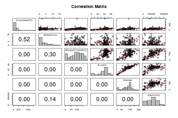
Title produced by software

Kendall tau Correlation Matrix

Date of computation

Fri, 23 Dec 2011 12:00:55 -0500

Cite this page as follows

Statistical Computations at FreeStatistics.org, Office for Research Development and Education, URL https://freestatistics.org/blog/index.php?v=date/2011/Dec/23/t13246596785mijrk3d5mrf5gl.htm/, Retrieved Mon, 29 Apr 2024 18:57:54 +0000

Statistical Computations at FreeStatistics.org, Office for Research Development and Education, URL https://freestatistics.org/blog/index.php?pk=160584, Retrieved Mon, 29 Apr 2024 18:57:54 +0000

QR Codes:

Paste this QR Code to cite your computation.

Original text written by user:

IsPrivate?

No (this computation is public)

User-defined keywords

Estimated Impact

Family? (F = Feedback message, R = changed R code, M = changed R Module, P = changed Parameters, D = changed Data)

-     [One-Way-Between-Groups ANOVA- Free Statistics Software (Calculator)] [] [2010-11-02 14:17:22] [b98453cac15ba1066b407e146608df68]
- RMPD  [Multiple Regression] [Paper - deel 3 - ...] [2011-12-23 16:13:52] [ae1339cb5a7cf28362d01e7220b4a16c]
- RMPD    [Kendall tau Correlation Matrix] [Paper - Deel 3 Ke...] [2011-12-23 16:54:13] [ae1339cb5a7cf28362d01e7220b4a16c]
- R  D        [Kendall tau Correlation Matrix] [Paper - deel3 - k...] [2011-12-23 17:00:55] [e598b5cd83fcb010b35e92a01f5e81e9] [Current]
-    D          [Kendall tau Correlation Matrix] [Paper - deel3 pea...] [2011-12-23 17:11:23] [ae1339cb5a7cf28362d01e7220b4a16c] 
-                 [Kendall tau Correlation Matrix] [Paper -D3 - kenda...] [2011-12-23 17:12:38] [ae1339cb5a7cf28362d01e7220b4a16c] 
- RM              [Recursive Partitioning (Regression Trees)] [REgressiontree - ...] [2011-12-23 17:13:56] [ae1339cb5a7cf28362d01e7220b4a16c] 
- RM              [Recursive Partitioning (Regression Trees)] [Regression tree w...] [2011-12-23 17:15:20] [ae1339cb5a7cf28362d01e7220b4a16c] 
- R                 [Recursive Partitioning (Regression Trees)] [deel 3 regression...] [2011-12-23 18:26:42] [ae1339cb5a7cf28362d01e7220b4a16c] 

Feedback Forum

Post a new message

Dataseries X:

Download CSV

Histogram

Boxplots

95	3	96	42	130	186099
68	4	75	38	143	113854
64	16	70	46	118	99776
139	2	134	42	146	106194
51	1	83	30	73	100792
46	3	8	35	89	47552
118	0	173	40	146	250931
46	0	1	18	22	6853
79	7	88	38	132	115466
76	0	104	37	92	110896
82	0	114	46	147	169351
66	7	125	60	203	94853
60	10	57	37	113	72591
117	4	139	55	171	101345
50	10	87	44	87	113713
133	0	176	63	208	165354
63	8	114	40	153	164263
100	4	121	43	97	135213
44	3	103	32	95	111669
65	8	135	52	197	134163
103	0	123	49	160	140303
103	1	99	41	148	150773
62	5	77	25	84	111848
70	9	103	57	227	102509
159	1	158	45	154	96785
78	0	116	42	151	116136
101	5	114	45	142	158376
73	0	150	43	148	153990
58	0	64	36	110	64057
147	0	150	45	149	230054
54	3	143	50	179	184531
84	6	50	50	149	114198
56	1	145	51	187	198299
45	4	56	42	153	33750
87	4	141	44	163	189723
87	0	83	42	127	100826
77	0	112	44	151	188355
72	2	79	40	100	104470
36	1	33	17	46	58391
51	2	152	43	156	164808
44	10	126	41	128	134097
75	10	97	41	111	80238
87	5	84	40	119	133252
97	6	68	49	148	54518
90	1	50	52	65	121850
860	2	101	42	134	79367
57	2	20	26	66	56968
99	1	107	59	201	106314
120	10	150	50	177	191889
76	3	129	50	156	104864
56	0	99	47	158	160792
20	0	8	4	7	15049
94	8	88	51	175	191179
21	5	21	18	61	25109
70	3	30	14	41	45824
133	1	102	41	133	129711
86	5	166	61	228	210012
224	6	132	40	140	194679
65	0	161	44	155	197680
86	12	90	40	141	81180
70	10	160	51	181	197765
148	12	139	29	75	214738
72	11	104	43	97	96252
59	8	103	42	142	124527
67	3	66	41	136	153242
58	0	163	30	87	145707
60	6	93	39	140	113963
105	10	85	51	169	134904
84	2	154	40	129	114268
63	5	143	29	92	94333
67	13	107	47	160	102204
39	6	22	23	67	23824
60	7	85	48	179	111563
94	2	101	38	90	91313
67	5	131	42	144	89770
96	4	140	46	144	100125
54	3	156	40	144	165278
54	6	81	45	134	181712
62	2	137	42	146	80906
71	0	102	41	121	75881
50	1	74	37	112	83963
117	1	161	47	145	175721
45	5	30	26	99	68580
61	2	120	48	96	136323
31	0	49	8	27	55792
175	0	121	27	77	25157
70	6	76	38	137	100922
284	1	85	41	151	118845
95	4	151	61	126	170492
72	1	165	45	159	81716
63	1	89	41	101	115750
75	3	168	42	144	105590
90	10	48	35	102	92795
89	1	149	36	135	82390
138	4	75	40	147	135599
68	5	107	40	155	127667
80	7	116	38	138	163073
65	0	181	43	113	211381
130	12	155	65	248	189944
85	13	165	33	116	226168
83	9	121	51	176	117495
89	0	176	45	140	195894
116	0	86	36	59	80684
43	4	13	19	64	19630
87	4	120	25	40	88634
80	0	117	44	98	139292
132	0	133	45	139	128602
59	0	169	44	135	135848
50	0	39	35	97	178377
87	0	125	46	142	106330
62	5	82	44	155	178303
70	1	148	45	115	116938
9	0	12	1	0	5841
54	0	146	40	103	106020
25	4	23	11	30	24610
113	0	87	51	130	74151
63	1	164	38	102	232241
2	0	4	0	0	6622
67	5	81	30	77	127097
22	0	18	8	9	13155
157	3	118	43	150	160501
79	7	76	48	163	91502
113	14	55	49	148	24469
50	3	62	32	94	88229
52	0	16	8	21	13983
113	3	98	43	151	80716
115	0	137	52	187	157384
78	0	50	53	171	122975
135	4	152	49	170	191469
120	0	163	48	145	231257
122	3	142	56	198	258287
54	0	80	45	152	122531
63	0	59	40	112	61394
162	4	94	48	173	86480
162	5	128	50	177	195791
107	16	63	43	153	18284
146	6	127	46	161	147581
77	5	60	40	115	72558
87	2	118	45	147	147341
192	1	110	46	124	114651
75	2	46	37	57	100187
131	9	96	45	144	130332
67	1	128	39	126	134218
37	3	41	21	78	10901
61	11	146	50	153	145758
127	5	147	55	196	75767
58	2	121	40	130	134969
71	1	185	48	159	169216
0	9	0	0	0	0
0	0	4	0	0	7953
0	0	0	0	0	0
0	0	0	0	0	0
0	1	0	0	0	0
0	0	0	0	0	0
72	2	85	46	94	105406
123	3	164	52	129	174586
0	0	0	0	0	0
0	0	0	0	0	0
0	0	7	0	0	4245
7	0	12	5	13	21509
3	0	0	1	4	7670
106	0	37	48	89	15673
0	0	0	0	0	0
53	2	62	34	71	75882

Summary of computational transaction
Raw Input	view raw input (R code)
Raw Output	view raw output of R engine
Computing time	1 seconds
R Server	'Gwilym Jenkins' @ jenkins.wessa.net

\begin{tabular}{lllllllll}
\hline
Summary of computational transaction \tabularnewline
Raw Input & view raw input (R code)  \tabularnewline
Raw Output & view raw output of R engine  \tabularnewline
Computing time & 1 seconds \tabularnewline
R Server & 'Gwilym Jenkins' @ jenkins.wessa.net \tabularnewline
\hline
\end{tabular}
%Source: https://freestatistics.org/blog/index.php?pk=160584&T=0

[TABLE]
[ROW][C]Summary of computational transaction[/C][/ROW]
[ROW][C]Raw Input[/C][C]view raw input (R code) [/C][/ROW]
[ROW][C]Raw Output[/C][C]view raw output of R engine [/C][/ROW]
[ROW][C]Computing time[/C][C]1 seconds[/C][/ROW]
[ROW][C]R Server[/C][C]'Gwilym Jenkins' @ jenkins.wessa.net[/C][/ROW]
[/TABLE]
Source: https://freestatistics.org/blog/index.php?pk=160584&T=0

Globally Unique Identifier (entire table): ba.freestatistics.org/blog/index.php?pk=160584&T=0

As an alternative you can also use a QR Code:

The GUIDs for individual cells are displayed in the table below:

Summary of computational transaction
Raw Input	view raw input (R code)
Raw Output	view raw output of R engine
Computing time	1 seconds
R Server	'Gwilym Jenkins' @ jenkins.wessa.net

Correlations for all pairs of data series (method=pearson)
	#CompViews(PR)	#SharedComp	#BloggedComputations	#LongPR	#Reviews	#SecinComp
#CompViews(PR)	1	0.051	0.319	0.378	0.359	0.256
#SharedComp	0.051	1	0.082	0.272	0.312	0.115
#BloggedComputations	0.319	0.082	1	0.731	0.725	0.785
#LongPR	0.378	0.272	0.731	1	0.919	0.684
#Reviews	0.359	0.312	0.725	0.919	1	0.676
#SecinComp	0.256	0.115	0.785	0.684	0.676	1

\begin{tabular}{lllllllll}
\hline
Correlations for all pairs of data series (method=pearson) \tabularnewline
  & #CompViews(PR) & #SharedComp & #BloggedComputations & #LongPR & #Reviews & #SecinComp \tabularnewline
#CompViews(PR) & 1 & 0.051 & 0.319 & 0.378 & 0.359 & 0.256 \tabularnewline
#SharedComp & 0.051 & 1 & 0.082 & 0.272 & 0.312 & 0.115 \tabularnewline
#BloggedComputations & 0.319 & 0.082 & 1 & 0.731 & 0.725 & 0.785 \tabularnewline
#LongPR & 0.378 & 0.272 & 0.731 & 1 & 0.919 & 0.684 \tabularnewline
#Reviews & 0.359 & 0.312 & 0.725 & 0.919 & 1 & 0.676 \tabularnewline
#SecinComp & 0.256 & 0.115 & 0.785 & 0.684 & 0.676 & 1 \tabularnewline
\hline
\end{tabular}
%Source: https://freestatistics.org/blog/index.php?pk=160584&T=1

[TABLE]
[ROW][C]Correlations for all pairs of data series (method=pearson)[/C][/ROW]
[ROW][C] [/C][C]#CompViews(PR)[/C][C]#SharedComp[/C][C]#BloggedComputations[/C][C]#LongPR[/C][C]#Reviews[/C][C]#SecinComp[/C][/ROW]
[ROW][C]#CompViews(PR)[/C][C]1[/C][C]0.051[/C][C]0.319[/C][C]0.378[/C][C]0.359[/C][C]0.256[/C][/ROW]
[ROW][C]#SharedComp[/C][C]0.051[/C][C]1[/C][C]0.082[/C][C]0.272[/C][C]0.312[/C][C]0.115[/C][/ROW]
[ROW][C]#BloggedComputations[/C][C]0.319[/C][C]0.082[/C][C]1[/C][C]0.731[/C][C]0.725[/C][C]0.785[/C][/ROW]
[ROW][C]#LongPR[/C][C]0.378[/C][C]0.272[/C][C]0.731[/C][C]1[/C][C]0.919[/C][C]0.684[/C][/ROW]
[ROW][C]#Reviews[/C][C]0.359[/C][C]0.312[/C][C]0.725[/C][C]0.919[/C][C]1[/C][C]0.676[/C][/ROW]
[ROW][C]#SecinComp[/C][C]0.256[/C][C]0.115[/C][C]0.785[/C][C]0.684[/C][C]0.676[/C][C]1[/C][/ROW]
[/TABLE]
Source: https://freestatistics.org/blog/index.php?pk=160584&T=1

Globally Unique Identifier (entire table): ba.freestatistics.org/blog/index.php?pk=160584&T=1

As an alternative you can also use a QR Code:

The GUIDs for individual cells are displayed in the table below:

Correlations for all pairs of data series (method=pearson)
	#CompViews(PR)	#SharedComp	#BloggedComputations	#LongPR	#Reviews	#SecinComp
#CompViews(PR)	1	0.051	0.319	0.378	0.359	0.256
#SharedComp	0.051	1	0.082	0.272	0.312	0.115
#BloggedComputations	0.319	0.082	1	0.731	0.725	0.785
#LongPR	0.378	0.272	0.731	1	0.919	0.684
#Reviews	0.359	0.312	0.725	0.919	1	0.676
#SecinComp	0.256	0.115	0.785	0.684	0.676	1

Correlations for all pairs of data series with p-values
pair	Pearson r	Spearman rho	Kendall tau
#CompViews(PR);#SharedComp	0.0507	0.1714	0.1208
p-value	(0.5195)	(0.0282)	(0.031)
#CompViews(PR);#BloggedComputations	0.319	0.5197	0.3753
p-value	(0)	(0)	(0)
#CompViews(PR);#LongPR	0.3785	0.5916	0.4444
p-value	(0)	(0)	(0)
#CompViews(PR);#Reviews	0.3586	0.5419	0.4032
p-value	(0)	(0)	(0)
#CompViews(PR);#SecinComp	0.2558	0.465	0.3344
p-value	(9e-04)	(0)	(0)
#SharedComp;#BloggedComputations	0.0817	0.0756	0.0505
p-value	(0.2985)	(0.3363)	(0.3662)
#SharedComp;#LongPR	0.2725	0.2371	0.1719
p-value	(4e-04)	(0.0022)	(0.0024)
#SharedComp;#Reviews	0.3122	0.3125	0.2268
p-value	(0)	(0)	(1e-04)
#SharedComp;#SecinComp	0.1152	0.138	0.0991
p-value	(0.1417)	(0.0781)	(0.0754)
#BloggedComputations;#LongPR	0.7306	0.5769	0.4343
p-value	(0)	(0)	(0)
#BloggedComputations;#Reviews	0.7255	0.6034	0.4438
p-value	(0)	(0)	(0)
#BloggedComputations;#SecinComp	0.7849	0.7307	0.5601
p-value	(0)	(0)	(0)
#LongPR;#Reviews	0.919	0.8299	0.6959
p-value	(0)	(0)	(0)
#LongPR;#SecinComp	0.6843	0.5637	0.4227
p-value	(0)	(0)	(0)
#Reviews;#SecinComp	0.6761	0.5903	0.438
p-value	(0)	(0)	(0)

\begin{tabular}{lllllllll}
\hline
Correlations for all pairs of data series with p-values \tabularnewline
pair & Pearson r & Spearman rho & Kendall tau \tabularnewline
#CompViews(PR);#SharedComp & 0.0507 & 0.1714 & 0.1208 \tabularnewline
p-value & (0.5195) & (0.0282) & (0.031) \tabularnewline
#CompViews(PR);#BloggedComputations & 0.319 & 0.5197 & 0.3753 \tabularnewline
p-value & (0) & (0) & (0) \tabularnewline
#CompViews(PR);#LongPR & 0.3785 & 0.5916 & 0.4444 \tabularnewline
p-value & (0) & (0) & (0) \tabularnewline
#CompViews(PR);#Reviews & 0.3586 & 0.5419 & 0.4032 \tabularnewline
p-value & (0) & (0) & (0) \tabularnewline
#CompViews(PR);#SecinComp & 0.2558 & 0.465 & 0.3344 \tabularnewline
p-value & (9e-04) & (0) & (0) \tabularnewline
#SharedComp;#BloggedComputations & 0.0817 & 0.0756 & 0.0505 \tabularnewline
p-value & (0.2985) & (0.3363) & (0.3662) \tabularnewline
#SharedComp;#LongPR & 0.2725 & 0.2371 & 0.1719 \tabularnewline
p-value & (4e-04) & (0.0022) & (0.0024) \tabularnewline
#SharedComp;#Reviews & 0.3122 & 0.3125 & 0.2268 \tabularnewline
p-value & (0) & (0) & (1e-04) \tabularnewline
#SharedComp;#SecinComp & 0.1152 & 0.138 & 0.0991 \tabularnewline
p-value & (0.1417) & (0.0781) & (0.0754) \tabularnewline
#BloggedComputations;#LongPR & 0.7306 & 0.5769 & 0.4343 \tabularnewline
p-value & (0) & (0) & (0) \tabularnewline
#BloggedComputations;#Reviews & 0.7255 & 0.6034 & 0.4438 \tabularnewline
p-value & (0) & (0) & (0) \tabularnewline
#BloggedComputations;#SecinComp & 0.7849 & 0.7307 & 0.5601 \tabularnewline
p-value & (0) & (0) & (0) \tabularnewline
#LongPR;#Reviews & 0.919 & 0.8299 & 0.6959 \tabularnewline
p-value & (0) & (0) & (0) \tabularnewline
#LongPR;#SecinComp & 0.6843 & 0.5637 & 0.4227 \tabularnewline
p-value & (0) & (0) & (0) \tabularnewline
#Reviews;#SecinComp & 0.6761 & 0.5903 & 0.438 \tabularnewline
p-value & (0) & (0) & (0) \tabularnewline
\hline
\end{tabular}
%Source: https://freestatistics.org/blog/index.php?pk=160584&T=2

[TABLE]
[ROW][C]Correlations for all pairs of data series with p-values[/C][/ROW]
[ROW][C]pair[/C][C]Pearson r[/C][C]Spearman rho[/C][C]Kendall tau[/C][/ROW]
[ROW][C]#CompViews(PR);#SharedComp[/C][C]0.0507[/C][C]0.1714[/C][C]0.1208[/C][/ROW]
[ROW][C]p-value[/C][C](0.5195)[/C][C](0.0282)[/C][C](0.031)[/C][/ROW]
[ROW][C]#CompViews(PR);#BloggedComputations[/C][C]0.319[/C][C]0.5197[/C][C]0.3753[/C][/ROW]
[ROW][C]p-value[/C][C](0)[/C][C](0)[/C][C](0)[/C][/ROW]
[ROW][C]#CompViews(PR);#LongPR[/C][C]0.3785[/C][C]0.5916[/C][C]0.4444[/C][/ROW]
[ROW][C]p-value[/C][C](0)[/C][C](0)[/C][C](0)[/C][/ROW]
[ROW][C]#CompViews(PR);#Reviews[/C][C]0.3586[/C][C]0.5419[/C][C]0.4032[/C][/ROW]
[ROW][C]p-value[/C][C](0)[/C][C](0)[/C][C](0)[/C][/ROW]
[ROW][C]#CompViews(PR);#SecinComp[/C][C]0.2558[/C][C]0.465[/C][C]0.3344[/C][/ROW]
[ROW][C]p-value[/C][C](9e-04)[/C][C](0)[/C][C](0)[/C][/ROW]
[ROW][C]#SharedComp;#BloggedComputations[/C][C]0.0817[/C][C]0.0756[/C][C]0.0505[/C][/ROW]
[ROW][C]p-value[/C][C](0.2985)[/C][C](0.3363)[/C][C](0.3662)[/C][/ROW]
[ROW][C]#SharedComp;#LongPR[/C][C]0.2725[/C][C]0.2371[/C][C]0.1719[/C][/ROW]
[ROW][C]p-value[/C][C](4e-04)[/C][C](0.0022)[/C][C](0.0024)[/C][/ROW]
[ROW][C]#SharedComp;#Reviews[/C][C]0.3122[/C][C]0.3125[/C][C]0.2268[/C][/ROW]
[ROW][C]p-value[/C][C](0)[/C][C](0)[/C][C](1e-04)[/C][/ROW]
[ROW][C]#SharedComp;#SecinComp[/C][C]0.1152[/C][C]0.138[/C][C]0.0991[/C][/ROW]
[ROW][C]p-value[/C][C](0.1417)[/C][C](0.0781)[/C][C](0.0754)[/C][/ROW]
[ROW][C]#BloggedComputations;#LongPR[/C][C]0.7306[/C][C]0.5769[/C][C]0.4343[/C][/ROW]
[ROW][C]p-value[/C][C](0)[/C][C](0)[/C][C](0)[/C][/ROW]
[ROW][C]#BloggedComputations;#Reviews[/C][C]0.7255[/C][C]0.6034[/C][C]0.4438[/C][/ROW]
[ROW][C]p-value[/C][C](0)[/C][C](0)[/C][C](0)[/C][/ROW]
[ROW][C]#BloggedComputations;#SecinComp[/C][C]0.7849[/C][C]0.7307[/C][C]0.5601[/C][/ROW]
[ROW][C]p-value[/C][C](0)[/C][C](0)[/C][C](0)[/C][/ROW]
[ROW][C]#LongPR;#Reviews[/C][C]0.919[/C][C]0.8299[/C][C]0.6959[/C][/ROW]
[ROW][C]p-value[/C][C](0)[/C][C](0)[/C][C](0)[/C][/ROW]
[ROW][C]#LongPR;#SecinComp[/C][C]0.6843[/C][C]0.5637[/C][C]0.4227[/C][/ROW]
[ROW][C]p-value[/C][C](0)[/C][C](0)[/C][C](0)[/C][/ROW]
[ROW][C]#Reviews;#SecinComp[/C][C]0.6761[/C][C]0.5903[/C][C]0.438[/C][/ROW]
[ROW][C]p-value[/C][C](0)[/C][C](0)[/C][C](0)[/C][/ROW]
[/TABLE]
Source: https://freestatistics.org/blog/index.php?pk=160584&T=2

Globally Unique Identifier (entire table): ba.freestatistics.org/blog/index.php?pk=160584&T=2

As an alternative you can also use a QR Code:

The GUIDs for individual cells are displayed in the table below:

Correlations for all pairs of data series with p-values
pair	Pearson r	Spearman rho	Kendall tau
#CompViews(PR);#SharedComp	0.0507	0.1714	0.1208
p-value	(0.5195)	(0.0282)	(0.031)
#CompViews(PR);#BloggedComputations	0.319	0.5197	0.3753
p-value	(0)	(0)	(0)
#CompViews(PR);#LongPR	0.3785	0.5916	0.4444
p-value	(0)	(0)	(0)
#CompViews(PR);#Reviews	0.3586	0.5419	0.4032
p-value	(0)	(0)	(0)
#CompViews(PR);#SecinComp	0.2558	0.465	0.3344
p-value	(9e-04)	(0)	(0)
#SharedComp;#BloggedComputations	0.0817	0.0756	0.0505
p-value	(0.2985)	(0.3363)	(0.3662)
#SharedComp;#LongPR	0.2725	0.2371	0.1719
p-value	(4e-04)	(0.0022)	(0.0024)
#SharedComp;#Reviews	0.3122	0.3125	0.2268
p-value	(0)	(0)	(1e-04)
#SharedComp;#SecinComp	0.1152	0.138	0.0991
p-value	(0.1417)	(0.0781)	(0.0754)
#BloggedComputations;#LongPR	0.7306	0.5769	0.4343
p-value	(0)	(0)	(0)
#BloggedComputations;#Reviews	0.7255	0.6034	0.4438
p-value	(0)	(0)	(0)
#BloggedComputations;#SecinComp	0.7849	0.7307	0.5601
p-value	(0)	(0)	(0)
#LongPR;#Reviews	0.919	0.8299	0.6959
p-value	(0)	(0)	(0)
#LongPR;#SecinComp	0.6843	0.5637	0.4227
p-value	(0)	(0)	(0)
#Reviews;#SecinComp	0.6761	0.5903	0.438
p-value	(0)	(0)	(0)

Figure 1

PNG link

Postscript link

PDF link

Parameters (Session):

par1 = 11 ; par2 = Do not include Seasonal Dummies ; par3 = No Linear Trend ;

Parameters (R input):

par1 = pearson ;

R code (references can be found in the software module):

panel.tau <- function(x, y, digits=2, prefix='', cex.cor)
{
usr <- par('usr'); on.exit(par(usr))
par(usr = c(0, 1, 0, 1))
rr <- cor.test(x, y, method=par1)
r <- round(rr$p.value,2)
txt <- format(c(r, 0.123456789), digits=digits)[1]
txt <- paste(prefix, txt, sep='')
if(missing(cex.cor)) cex <- 0.5/strwidth(txt)
text(0.5, 0.5, txt, cex = cex)
}
panel.hist <- function(x, ...)
{
usr <- par('usr'); on.exit(par(usr))
par(usr = c(usr[1:2], 0, 1.5) )
h <- hist(x, plot = FALSE)
breaks <- h$breaks; nB <- length(breaks)
y <- h$counts; y <- y/max(y)
rect(breaks[-nB], 0, breaks[-1], y, col='grey', ...)
}
bitmap(file='test1.png')
pairs(t(y),diag.panel=panel.hist, upper.panel=panel.smooth, lower.panel=panel.tau, main=main)
dev.off()
load(file='createtable')
n <- length(y[,1])
n
a<-table.start()
a<-table.row.start(a)
a<-table.element(a,paste('Correlations for all pairs of data series (method=',par1,')',sep=''),n+1,TRUE)
a<-table.row.end(a)
a<-table.row.start(a)
a<-table.element(a,' ',header=TRUE)
for (i in 1:n) {
a<-table.element(a,dimnames(t(x))[[2]][i],header=TRUE)
}
a<-table.row.end(a)
for (i in 1:n) {
a<-table.row.start(a)
a<-table.element(a,dimnames(t(x))[[2]][i],header=TRUE)
for (j in 1:n) {
r <- cor.test(y[i,],y[j,],method=par1)
a<-table.element(a,round(r$estimate,3))
}
a<-table.row.end(a)
}
a<-table.end(a)
table.save(a,file='mytable.tab')
a<-table.start()
a<-table.row.start(a)
a<-table.element(a,'Correlations for all pairs of data series with p-values',4,TRUE)
a<-table.row.end(a)
a<-table.row.start(a)
a<-table.element(a,'pair',1,TRUE)
a<-table.element(a,'Pearson r',1,TRUE)
a<-table.element(a,'Spearman rho',1,TRUE)
a<-table.element(a,'Kendall tau',1,TRUE)
a<-table.row.end(a)
cor.test(y[1,],y[2,],method=par1)
for (i in 1:(n-1))
{
for (j in (i+1):n)
{
a<-table.row.start(a)
dum <- paste(dimnames(t(x))[[2]][i],';',dimnames(t(x))[[2]][j],sep='')
a<-table.element(a,dum,header=TRUE)
rp <- cor.test(y[i,],y[j,],method='pearson')
a<-table.element(a,round(rp$estimate,4))
rs <- cor.test(y[i,],y[j,],method='spearman')
a<-table.element(a,round(rs$estimate,4))
rk <- cor.test(y[i,],y[j,],method='kendall')
a<-table.element(a,round(rk$estimate,4))
a<-table.row.end(a)
a<-table.row.start(a)
a<-table.element(a,'p-value',header=T)
a<-table.element(a,paste('(',round(rp$p.value,4),')',sep=''))
a<-table.element(a,paste('(',round(rs$p.value,4),')',sep=''))
a<-table.element(a,paste('(',round(rk$p.value,4),')',sep=''))
a<-table.row.end(a)
}
}
a<-table.end(a)
table.save(a,file='mytable1.tab')

Free Statistics

Description of Statistical Computation

Tree of Dependent Computations

Dataset

Tables (Output of Computation)

Figures (Output of Computation)

Input Parameters & R Code