Repository of Reproducible Computations

Free Statistics

of Irreproducible Research!

Author's title

Author

*The author of this computation has been verified*

R Software Module

rwasp_autocorrelation.wasp

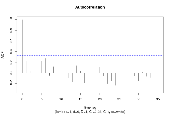
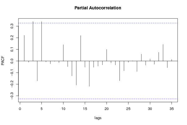
Title produced by software

(Partial) Autocorrelation Function

Date of computation

Fri, 23 Dec 2011 09:14:36 -0500

Cite this page as follows

Statistical Computations at FreeStatistics.org, Office for Research Development and Education, URL https://freestatistics.org/blog/index.php?v=date/2011/Dec/23/t1324649686ry8pt8o7zj60qjg.htm/, Retrieved Mon, 29 Apr 2024 21:56:28 +0000

Statistical Computations at FreeStatistics.org, Office for Research Development and Education, URL https://freestatistics.org/blog/index.php?pk=160432, Retrieved Mon, 29 Apr 2024 21:56:28 +0000

QR Codes:

Paste this QR Code to cite your computation.

Original text written by user:

IsPrivate?

No (this computation is public)

User-defined keywords

Estimated Impact

Family? (F = Feedback message, R = changed R code, M = changed R Module, P = changed Parameters, D = changed Data)

-     [Univariate Explorative Data Analysis] [Run Sequence gebo...] [2008-12-12 13:32:37] [76963dc1903f0f612b6153510a3818cf]
- R  D  [Univariate Explorative Data Analysis] [Run Sequence gebo...] [2008-12-17 12:14:40] [76963dc1903f0f612b6153510a3818cf]
-         [Univariate Explorative Data Analysis] [Run Sequence Plot...] [2008-12-22 18:19:51] [1ce0d16c8f4225c977b42c8fa93bc163]
- RMP       [Univariate Data Series] [Identifying Integ...] [2009-11-22 12:08:06] [b98453cac15ba1066b407e146608df68]
- RMP         [(Partial) Autocorrelation Function] [Births] [2010-11-29 09:36:27] [b98453cac15ba1066b407e146608df68]
-   PD          [(Partial) Autocorrelation Function] [ WS 9 : ACF - d=0...] [2010-12-08 10:48:57] [2c786c21adba4dd4c8af44dce5258f06]
-   P             [(Partial) Autocorrelation Function] [ws 9 : ACF d=0 D=1 ] [2010-12-08 11:00:09] [2c786c21adba4dd4c8af44dce5258f06]
-   P               [(Partial) Autocorrelation Function] [ws 9 : ACF d=0 D=...] [2010-12-08 14:54:21] [2c786c21adba4dd4c8af44dce5258f06]
- R PD                  [(Partial) Autocorrelation Function] [] [2011-12-23 14:14:36] [c80accbb627afb8a1e74b91ef6a0d2c4] [Current]

Feedback Forum

Post a new message

Dataseries X:

Download CSV

Histogram

Boxplots

Summary of computational transaction
Raw Input	view raw input (R code)
Raw Output	view raw output of R engine
Computing time	2 seconds
R Server	'AstonUniversity' @ aston.wessa.net

\begin{tabular}{lllllllll}
\hline
Summary of computational transaction \tabularnewline
Raw Input & view raw input (R code)  \tabularnewline
Raw Output & view raw output of R engine  \tabularnewline
Computing time & 2 seconds \tabularnewline
R Server & 'AstonUniversity' @ aston.wessa.net \tabularnewline
\hline
\end{tabular}
%Source: https://freestatistics.org/blog/index.php?pk=160432&T=0

[TABLE]
[ROW][C]Summary of computational transaction[/C][/ROW]
[ROW][C]Raw Input[/C][C]view raw input (R code) [/C][/ROW]
[ROW][C]Raw Output[/C][C]view raw output of R engine [/C][/ROW]
[ROW][C]Computing time[/C][C]2 seconds[/C][/ROW]
[ROW][C]R Server[/C][C]'AstonUniversity' @ aston.wessa.net[/C][/ROW]
[/TABLE]
Source: https://freestatistics.org/blog/index.php?pk=160432&T=0

Globally Unique Identifier (entire table): ba.freestatistics.org/blog/index.php?pk=160432&T=0

As an alternative you can also use a QR Code:

The GUIDs for individual cells are displayed in the table below:

Summary of computational transaction
Raw Input	view raw input (R code)
Raw Output	view raw output of R engine
Computing time	2 seconds
R Server	'AstonUniversity' @ aston.wessa.net

Autocorrelation Function
Time lag k	ACF(k)	T-STAT	P-value
1	0.22143	1.3286	0.096174
2	0.039196	0.2352	0.407702
3	0.329598	1.9776	0.027835
4	0.002711	0.0163	0.493555
5	0.221107	1.3266	0.09649
6	0.270696	1.6242	0.056532
7	-0.050656	-0.3039	0.381462
8	0.115687	0.6941	0.24603
9	0.094395	0.5664	0.287329
10	0.080503	0.483	0.316005
11	0.159728	0.9584	0.172135
12	-0.09256	-0.5554	0.291041
13	-0.169438	-1.0166	0.158058
14	0.135786	0.8147	0.210295
15	0.035996	0.216	0.415113
16	-0.190588	-1.1435	0.130183
17	-0.064353	-0.3861	0.350842
18	-0.14891	-0.8935	0.188773
19	-0.187577	-1.1255	0.133921
20	0.112064	0.6724	0.252815
21	-0.057505	-0.345	0.36604
22	-0.202523	-1.2151	0.116111
23	-0.148336	-0.89	0.189683
24	-0.233816	-1.4029	0.084607
25	-0.066322	-0.3979	0.346515
26	-0.061257	-0.3675	0.357684
27	-0.296744	-1.7805	0.041721
28	-0.064508	-0.387	0.3505
29	-0.056173	-0.337	0.369022
30	-0.155206	-0.9312	0.178967
31	0.015448	0.0927	0.463332
32	-0.065708	-0.3943	0.347861
33	-0.089092	-0.5346	0.298122
34	0.039954	0.2397	0.405952
35	0.026971	0.1618	0.436174
36	NA	NA	NA
37	NA	NA	NA
38	NA	NA	NA
39	NA	NA	NA
40	NA	NA	NA
41	NA	NA	NA
42	NA	NA	NA
43	NA	NA	NA
44	NA	NA	NA
45	NA	NA	NA
46	NA	NA	NA
47	NA	NA	NA
48	NA	NA	NA

\begin{tabular}{lllllllll}
\hline
Autocorrelation Function \tabularnewline
Time lag k & ACF(k) & T-STAT & P-value \tabularnewline
1 & 0.22143 & 1.3286 & 0.096174 \tabularnewline
2 & 0.039196 & 0.2352 & 0.407702 \tabularnewline
3 & 0.329598 & 1.9776 & 0.027835 \tabularnewline
4 & 0.002711 & 0.0163 & 0.493555 \tabularnewline
5 & 0.221107 & 1.3266 & 0.09649 \tabularnewline
6 & 0.270696 & 1.6242 & 0.056532 \tabularnewline
7 & -0.050656 & -0.3039 & 0.381462 \tabularnewline
8 & 0.115687 & 0.6941 & 0.24603 \tabularnewline
9 & 0.094395 & 0.5664 & 0.287329 \tabularnewline
10 & 0.080503 & 0.483 & 0.316005 \tabularnewline
11 & 0.159728 & 0.9584 & 0.172135 \tabularnewline
12 & -0.09256 & -0.5554 & 0.291041 \tabularnewline
13 & -0.169438 & -1.0166 & 0.158058 \tabularnewline
14 & 0.135786 & 0.8147 & 0.210295 \tabularnewline
15 & 0.035996 & 0.216 & 0.415113 \tabularnewline
16 & -0.190588 & -1.1435 & 0.130183 \tabularnewline
17 & -0.064353 & -0.3861 & 0.350842 \tabularnewline
18 & -0.14891 & -0.8935 & 0.188773 \tabularnewline
19 & -0.187577 & -1.1255 & 0.133921 \tabularnewline
20 & 0.112064 & 0.6724 & 0.252815 \tabularnewline
21 & -0.057505 & -0.345 & 0.36604 \tabularnewline
22 & -0.202523 & -1.2151 & 0.116111 \tabularnewline
23 & -0.148336 & -0.89 & 0.189683 \tabularnewline
24 & -0.233816 & -1.4029 & 0.084607 \tabularnewline
25 & -0.066322 & -0.3979 & 0.346515 \tabularnewline
26 & -0.061257 & -0.3675 & 0.357684 \tabularnewline
27 & -0.296744 & -1.7805 & 0.041721 \tabularnewline
28 & -0.064508 & -0.387 & 0.3505 \tabularnewline
29 & -0.056173 & -0.337 & 0.369022 \tabularnewline
30 & -0.155206 & -0.9312 & 0.178967 \tabularnewline
31 & 0.015448 & 0.0927 & 0.463332 \tabularnewline
32 & -0.065708 & -0.3943 & 0.347861 \tabularnewline
33 & -0.089092 & -0.5346 & 0.298122 \tabularnewline
34 & 0.039954 & 0.2397 & 0.405952 \tabularnewline
35 & 0.026971 & 0.1618 & 0.436174 \tabularnewline
36 & NA & NA & NA \tabularnewline
37 & NA & NA & NA \tabularnewline
38 & NA & NA & NA \tabularnewline
39 & NA & NA & NA \tabularnewline
40 & NA & NA & NA \tabularnewline
41 & NA & NA & NA \tabularnewline
42 & NA & NA & NA \tabularnewline
43 & NA & NA & NA \tabularnewline
44 & NA & NA & NA \tabularnewline
45 & NA & NA & NA \tabularnewline
46 & NA & NA & NA \tabularnewline
47 & NA & NA & NA \tabularnewline
48 & NA & NA & NA \tabularnewline
\hline
\end{tabular}
%Source: https://freestatistics.org/blog/index.php?pk=160432&T=1

[TABLE]
[ROW][C]Autocorrelation Function[/C][/ROW]
[ROW][C]Time lag k[/C][C]ACF(k)[/C][C]T-STAT[/C][C]P-value[/C][/ROW]
[ROW][C]1[/C][C]0.22143[/C][C]1.3286[/C][C]0.096174[/C][/ROW]
[ROW][C]2[/C][C]0.039196[/C][C]0.2352[/C][C]0.407702[/C][/ROW]
[ROW][C]3[/C][C]0.329598[/C][C]1.9776[/C][C]0.027835[/C][/ROW]
[ROW][C]4[/C][C]0.002711[/C][C]0.0163[/C][C]0.493555[/C][/ROW]
[ROW][C]5[/C][C]0.221107[/C][C]1.3266[/C][C]0.09649[/C][/ROW]
[ROW][C]6[/C][C]0.270696[/C][C]1.6242[/C][C]0.056532[/C][/ROW]
[ROW][C]7[/C][C]-0.050656[/C][C]-0.3039[/C][C]0.381462[/C][/ROW]
[ROW][C]8[/C][C]0.115687[/C][C]0.6941[/C][C]0.24603[/C][/ROW]
[ROW][C]9[/C][C]0.094395[/C][C]0.5664[/C][C]0.287329[/C][/ROW]
[ROW][C]10[/C][C]0.080503[/C][C]0.483[/C][C]0.316005[/C][/ROW]
[ROW][C]11[/C][C]0.159728[/C][C]0.9584[/C][C]0.172135[/C][/ROW]
[ROW][C]12[/C][C]-0.09256[/C][C]-0.5554[/C][C]0.291041[/C][/ROW]
[ROW][C]13[/C][C]-0.169438[/C][C]-1.0166[/C][C]0.158058[/C][/ROW]
[ROW][C]14[/C][C]0.135786[/C][C]0.8147[/C][C]0.210295[/C][/ROW]
[ROW][C]15[/C][C]0.035996[/C][C]0.216[/C][C]0.415113[/C][/ROW]
[ROW][C]16[/C][C]-0.190588[/C][C]-1.1435[/C][C]0.130183[/C][/ROW]
[ROW][C]17[/C][C]-0.064353[/C][C]-0.3861[/C][C]0.350842[/C][/ROW]
[ROW][C]18[/C][C]-0.14891[/C][C]-0.8935[/C][C]0.188773[/C][/ROW]
[ROW][C]19[/C][C]-0.187577[/C][C]-1.1255[/C][C]0.133921[/C][/ROW]
[ROW][C]20[/C][C]0.112064[/C][C]0.6724[/C][C]0.252815[/C][/ROW]
[ROW][C]21[/C][C]-0.057505[/C][C]-0.345[/C][C]0.36604[/C][/ROW]
[ROW][C]22[/C][C]-0.202523[/C][C]-1.2151[/C][C]0.116111[/C][/ROW]
[ROW][C]23[/C][C]-0.148336[/C][C]-0.89[/C][C]0.189683[/C][/ROW]
[ROW][C]24[/C][C]-0.233816[/C][C]-1.4029[/C][C]0.084607[/C][/ROW]
[ROW][C]25[/C][C]-0.066322[/C][C]-0.3979[/C][C]0.346515[/C][/ROW]
[ROW][C]26[/C][C]-0.061257[/C][C]-0.3675[/C][C]0.357684[/C][/ROW]
[ROW][C]27[/C][C]-0.296744[/C][C]-1.7805[/C][C]0.041721[/C][/ROW]
[ROW][C]28[/C][C]-0.064508[/C][C]-0.387[/C][C]0.3505[/C][/ROW]
[ROW][C]29[/C][C]-0.056173[/C][C]-0.337[/C][C]0.369022[/C][/ROW]
[ROW][C]30[/C][C]-0.155206[/C][C]-0.9312[/C][C]0.178967[/C][/ROW]
[ROW][C]31[/C][C]0.015448[/C][C]0.0927[/C][C]0.463332[/C][/ROW]
[ROW][C]32[/C][C]-0.065708[/C][C]-0.3943[/C][C]0.347861[/C][/ROW]
[ROW][C]33[/C][C]-0.089092[/C][C]-0.5346[/C][C]0.298122[/C][/ROW]
[ROW][C]34[/C][C]0.039954[/C][C]0.2397[/C][C]0.405952[/C][/ROW]
[ROW][C]35[/C][C]0.026971[/C][C]0.1618[/C][C]0.436174[/C][/ROW]
[ROW][C]36[/C][C]NA[/C][C]NA[/C][C]NA[/C][/ROW]
[ROW][C]37[/C][C]NA[/C][C]NA[/C][C]NA[/C][/ROW]
[ROW][C]38[/C][C]NA[/C][C]NA[/C][C]NA[/C][/ROW]
[ROW][C]39[/C][C]NA[/C][C]NA[/C][C]NA[/C][/ROW]
[ROW][C]40[/C][C]NA[/C][C]NA[/C][C]NA[/C][/ROW]
[ROW][C]41[/C][C]NA[/C][C]NA[/C][C]NA[/C][/ROW]
[ROW][C]42[/C][C]NA[/C][C]NA[/C][C]NA[/C][/ROW]
[ROW][C]43[/C][C]NA[/C][C]NA[/C][C]NA[/C][/ROW]
[ROW][C]44[/C][C]NA[/C][C]NA[/C][C]NA[/C][/ROW]
[ROW][C]45[/C][C]NA[/C][C]NA[/C][C]NA[/C][/ROW]
[ROW][C]46[/C][C]NA[/C][C]NA[/C][C]NA[/C][/ROW]
[ROW][C]47[/C][C]NA[/C][C]NA[/C][C]NA[/C][/ROW]
[ROW][C]48[/C][C]NA[/C][C]NA[/C][C]NA[/C][/ROW]
[/TABLE]
Source: https://freestatistics.org/blog/index.php?pk=160432&T=1

Globally Unique Identifier (entire table): ba.freestatistics.org/blog/index.php?pk=160432&T=1

As an alternative you can also use a QR Code:

The GUIDs for individual cells are displayed in the table below:

Autocorrelation Function
Time lag k	ACF(k)	T-STAT	P-value
1	0.22143	1.3286	0.096174
2	0.039196	0.2352	0.407702
3	0.329598	1.9776	0.027835
4	0.002711	0.0163	0.493555
5	0.221107	1.3266	0.09649
6	0.270696	1.6242	0.056532
7	-0.050656	-0.3039	0.381462
8	0.115687	0.6941	0.24603
9	0.094395	0.5664	0.287329
10	0.080503	0.483	0.316005
11	0.159728	0.9584	0.172135
12	-0.09256	-0.5554	0.291041
13	-0.169438	-1.0166	0.158058
14	0.135786	0.8147	0.210295
15	0.035996	0.216	0.415113
16	-0.190588	-1.1435	0.130183
17	-0.064353	-0.3861	0.350842
18	-0.14891	-0.8935	0.188773
19	-0.187577	-1.1255	0.133921
20	0.112064	0.6724	0.252815
21	-0.057505	-0.345	0.36604
22	-0.202523	-1.2151	0.116111
23	-0.148336	-0.89	0.189683
24	-0.233816	-1.4029	0.084607
25	-0.066322	-0.3979	0.346515
26	-0.061257	-0.3675	0.357684
27	-0.296744	-1.7805	0.041721
28	-0.064508	-0.387	0.3505
29	-0.056173	-0.337	0.369022
30	-0.155206	-0.9312	0.178967
31	0.015448	0.0927	0.463332
32	-0.065708	-0.3943	0.347861
33	-0.089092	-0.5346	0.298122
34	0.039954	0.2397	0.405952
35	0.026971	0.1618	0.436174
36	NA	NA	NA
37	NA	NA	NA
38	NA	NA	NA
39	NA	NA	NA
40	NA	NA	NA
41	NA	NA	NA
42	NA	NA	NA
43	NA	NA	NA
44	NA	NA	NA
45	NA	NA	NA
46	NA	NA	NA
47	NA	NA	NA
48	NA	NA	NA

Partial Autocorrelation Function
Time lag k	PACF(k)	T-STAT	P-value
1	0.22143	1.3286	0.096174
2	-0.010342	-0.0621	0.475433
3	0.339815	2.0389	0.024428
4	-0.171264	-1.0276	0.1555
5	0.338993	2.034	0.024688
6	-0.007361	-0.0442	0.482509
7	-0.023681	-0.1421	0.443901
8	-0.002407	-0.0144	0.494279
9	-0.013885	-0.0833	0.467034
10	0.14071	0.8443	0.20205
11	-0.048753	-0.2925	0.385786
12	-0.128277	-0.7697	0.223262
13	-0.20733	-1.244	0.110773
14	0.219295	1.3158	0.098284
15	-0.053434	-0.3206	0.375182
16	-0.217929	-1.3076	0.099653
17	-0.054044	-0.3243	0.373809
18	-0.044012	-0.2641	0.396615
19	-0.033426	-0.2006	0.421087
20	0.099876	0.5993	0.276378
21	-0.016768	-0.1006	0.46021
22	-0.034054	-0.2043	0.419626
23	-0.169863	-1.0192	0.157459
24	-0.084332	-0.506	0.307974
25	-0.010708	-0.0642	0.474563
26	0.001166	0.007	0.497228
27	-0.090088	-0.5405	0.296081
28	0.058996	0.354	0.36271
29	-0.0356	-0.2136	0.416033
30	0.018244	0.1095	0.456721
31	-0.028403	-0.1704	0.432817
32	0.074954	0.4497	0.327802
33	0.142355	0.8541	0.19934
34	-0.057391	-0.3443	0.366295
35	0.013537	0.0812	0.467857
36	NA	NA	NA
37	NA	NA	NA
38	NA	NA	NA
39	NA	NA	NA
40	NA	NA	NA
41	NA	NA	NA
42	NA	NA	NA
43	NA	NA	NA
44	NA	NA	NA
45	NA	NA	NA
46	NA	NA	NA
47	NA	NA	NA
48	NA	NA	NA

\begin{tabular}{lllllllll}
\hline
Partial Autocorrelation Function \tabularnewline
Time lag k & PACF(k) & T-STAT & P-value \tabularnewline
1 & 0.22143 & 1.3286 & 0.096174 \tabularnewline
2 & -0.010342 & -0.0621 & 0.475433 \tabularnewline
3 & 0.339815 & 2.0389 & 0.024428 \tabularnewline
4 & -0.171264 & -1.0276 & 0.1555 \tabularnewline
5 & 0.338993 & 2.034 & 0.024688 \tabularnewline
6 & -0.007361 & -0.0442 & 0.482509 \tabularnewline
7 & -0.023681 & -0.1421 & 0.443901 \tabularnewline
8 & -0.002407 & -0.0144 & 0.494279 \tabularnewline
9 & -0.013885 & -0.0833 & 0.467034 \tabularnewline
10 & 0.14071 & 0.8443 & 0.20205 \tabularnewline
11 & -0.048753 & -0.2925 & 0.385786 \tabularnewline
12 & -0.128277 & -0.7697 & 0.223262 \tabularnewline
13 & -0.20733 & -1.244 & 0.110773 \tabularnewline
14 & 0.219295 & 1.3158 & 0.098284 \tabularnewline
15 & -0.053434 & -0.3206 & 0.375182 \tabularnewline
16 & -0.217929 & -1.3076 & 0.099653 \tabularnewline
17 & -0.054044 & -0.3243 & 0.373809 \tabularnewline
18 & -0.044012 & -0.2641 & 0.396615 \tabularnewline
19 & -0.033426 & -0.2006 & 0.421087 \tabularnewline
20 & 0.099876 & 0.5993 & 0.276378 \tabularnewline
21 & -0.016768 & -0.1006 & 0.46021 \tabularnewline
22 & -0.034054 & -0.2043 & 0.419626 \tabularnewline
23 & -0.169863 & -1.0192 & 0.157459 \tabularnewline
24 & -0.084332 & -0.506 & 0.307974 \tabularnewline
25 & -0.010708 & -0.0642 & 0.474563 \tabularnewline
26 & 0.001166 & 0.007 & 0.497228 \tabularnewline
27 & -0.090088 & -0.5405 & 0.296081 \tabularnewline
28 & 0.058996 & 0.354 & 0.36271 \tabularnewline
29 & -0.0356 & -0.2136 & 0.416033 \tabularnewline
30 & 0.018244 & 0.1095 & 0.456721 \tabularnewline
31 & -0.028403 & -0.1704 & 0.432817 \tabularnewline
32 & 0.074954 & 0.4497 & 0.327802 \tabularnewline
33 & 0.142355 & 0.8541 & 0.19934 \tabularnewline
34 & -0.057391 & -0.3443 & 0.366295 \tabularnewline
35 & 0.013537 & 0.0812 & 0.467857 \tabularnewline
36 & NA & NA & NA \tabularnewline
37 & NA & NA & NA \tabularnewline
38 & NA & NA & NA \tabularnewline
39 & NA & NA & NA \tabularnewline
40 & NA & NA & NA \tabularnewline
41 & NA & NA & NA \tabularnewline
42 & NA & NA & NA \tabularnewline
43 & NA & NA & NA \tabularnewline
44 & NA & NA & NA \tabularnewline
45 & NA & NA & NA \tabularnewline
46 & NA & NA & NA \tabularnewline
47 & NA & NA & NA \tabularnewline
48 & NA & NA & NA \tabularnewline
\hline
\end{tabular}
%Source: https://freestatistics.org/blog/index.php?pk=160432&T=2

[TABLE]
[ROW][C]Partial Autocorrelation Function[/C][/ROW]
[ROW][C]Time lag k[/C][C]PACF(k)[/C][C]T-STAT[/C][C]P-value[/C][/ROW]
[ROW][C]1[/C][C]0.22143[/C][C]1.3286[/C][C]0.096174[/C][/ROW]
[ROW][C]2[/C][C]-0.010342[/C][C]-0.0621[/C][C]0.475433[/C][/ROW]
[ROW][C]3[/C][C]0.339815[/C][C]2.0389[/C][C]0.024428[/C][/ROW]
[ROW][C]4[/C][C]-0.171264[/C][C]-1.0276[/C][C]0.1555[/C][/ROW]
[ROW][C]5[/C][C]0.338993[/C][C]2.034[/C][C]0.024688[/C][/ROW]
[ROW][C]6[/C][C]-0.007361[/C][C]-0.0442[/C][C]0.482509[/C][/ROW]
[ROW][C]7[/C][C]-0.023681[/C][C]-0.1421[/C][C]0.443901[/C][/ROW]
[ROW][C]8[/C][C]-0.002407[/C][C]-0.0144[/C][C]0.494279[/C][/ROW]
[ROW][C]9[/C][C]-0.013885[/C][C]-0.0833[/C][C]0.467034[/C][/ROW]
[ROW][C]10[/C][C]0.14071[/C][C]0.8443[/C][C]0.20205[/C][/ROW]
[ROW][C]11[/C][C]-0.048753[/C][C]-0.2925[/C][C]0.385786[/C][/ROW]
[ROW][C]12[/C][C]-0.128277[/C][C]-0.7697[/C][C]0.223262[/C][/ROW]
[ROW][C]13[/C][C]-0.20733[/C][C]-1.244[/C][C]0.110773[/C][/ROW]
[ROW][C]14[/C][C]0.219295[/C][C]1.3158[/C][C]0.098284[/C][/ROW]
[ROW][C]15[/C][C]-0.053434[/C][C]-0.3206[/C][C]0.375182[/C][/ROW]
[ROW][C]16[/C][C]-0.217929[/C][C]-1.3076[/C][C]0.099653[/C][/ROW]
[ROW][C]17[/C][C]-0.054044[/C][C]-0.3243[/C][C]0.373809[/C][/ROW]
[ROW][C]18[/C][C]-0.044012[/C][C]-0.2641[/C][C]0.396615[/C][/ROW]
[ROW][C]19[/C][C]-0.033426[/C][C]-0.2006[/C][C]0.421087[/C][/ROW]
[ROW][C]20[/C][C]0.099876[/C][C]0.5993[/C][C]0.276378[/C][/ROW]
[ROW][C]21[/C][C]-0.016768[/C][C]-0.1006[/C][C]0.46021[/C][/ROW]
[ROW][C]22[/C][C]-0.034054[/C][C]-0.2043[/C][C]0.419626[/C][/ROW]
[ROW][C]23[/C][C]-0.169863[/C][C]-1.0192[/C][C]0.157459[/C][/ROW]
[ROW][C]24[/C][C]-0.084332[/C][C]-0.506[/C][C]0.307974[/C][/ROW]
[ROW][C]25[/C][C]-0.010708[/C][C]-0.0642[/C][C]0.474563[/C][/ROW]
[ROW][C]26[/C][C]0.001166[/C][C]0.007[/C][C]0.497228[/C][/ROW]
[ROW][C]27[/C][C]-0.090088[/C][C]-0.5405[/C][C]0.296081[/C][/ROW]
[ROW][C]28[/C][C]0.058996[/C][C]0.354[/C][C]0.36271[/C][/ROW]
[ROW][C]29[/C][C]-0.0356[/C][C]-0.2136[/C][C]0.416033[/C][/ROW]
[ROW][C]30[/C][C]0.018244[/C][C]0.1095[/C][C]0.456721[/C][/ROW]
[ROW][C]31[/C][C]-0.028403[/C][C]-0.1704[/C][C]0.432817[/C][/ROW]
[ROW][C]32[/C][C]0.074954[/C][C]0.4497[/C][C]0.327802[/C][/ROW]
[ROW][C]33[/C][C]0.142355[/C][C]0.8541[/C][C]0.19934[/C][/ROW]
[ROW][C]34[/C][C]-0.057391[/C][C]-0.3443[/C][C]0.366295[/C][/ROW]
[ROW][C]35[/C][C]0.013537[/C][C]0.0812[/C][C]0.467857[/C][/ROW]
[ROW][C]36[/C][C]NA[/C][C]NA[/C][C]NA[/C][/ROW]
[ROW][C]37[/C][C]NA[/C][C]NA[/C][C]NA[/C][/ROW]
[ROW][C]38[/C][C]NA[/C][C]NA[/C][C]NA[/C][/ROW]
[ROW][C]39[/C][C]NA[/C][C]NA[/C][C]NA[/C][/ROW]
[ROW][C]40[/C][C]NA[/C][C]NA[/C][C]NA[/C][/ROW]
[ROW][C]41[/C][C]NA[/C][C]NA[/C][C]NA[/C][/ROW]
[ROW][C]42[/C][C]NA[/C][C]NA[/C][C]NA[/C][/ROW]
[ROW][C]43[/C][C]NA[/C][C]NA[/C][C]NA[/C][/ROW]
[ROW][C]44[/C][C]NA[/C][C]NA[/C][C]NA[/C][/ROW]
[ROW][C]45[/C][C]NA[/C][C]NA[/C][C]NA[/C][/ROW]
[ROW][C]46[/C][C]NA[/C][C]NA[/C][C]NA[/C][/ROW]
[ROW][C]47[/C][C]NA[/C][C]NA[/C][C]NA[/C][/ROW]
[ROW][C]48[/C][C]NA[/C][C]NA[/C][C]NA[/C][/ROW]
[/TABLE]
Source: https://freestatistics.org/blog/index.php?pk=160432&T=2

Globally Unique Identifier (entire table): ba.freestatistics.org/blog/index.php?pk=160432&T=2

As an alternative you can also use a QR Code:

The GUIDs for individual cells are displayed in the table below:

Partial Autocorrelation Function
Time lag k	PACF(k)	T-STAT	P-value
1	0.22143	1.3286	0.096174
2	-0.010342	-0.0621	0.475433
3	0.339815	2.0389	0.024428
4	-0.171264	-1.0276	0.1555
5	0.338993	2.034	0.024688
6	-0.007361	-0.0442	0.482509
7	-0.023681	-0.1421	0.443901
8	-0.002407	-0.0144	0.494279
9	-0.013885	-0.0833	0.467034
10	0.14071	0.8443	0.20205
11	-0.048753	-0.2925	0.385786
12	-0.128277	-0.7697	0.223262
13	-0.20733	-1.244	0.110773
14	0.219295	1.3158	0.098284
15	-0.053434	-0.3206	0.375182
16	-0.217929	-1.3076	0.099653
17	-0.054044	-0.3243	0.373809
18	-0.044012	-0.2641	0.396615
19	-0.033426	-0.2006	0.421087
20	0.099876	0.5993	0.276378
21	-0.016768	-0.1006	0.46021
22	-0.034054	-0.2043	0.419626
23	-0.169863	-1.0192	0.157459
24	-0.084332	-0.506	0.307974
25	-0.010708	-0.0642	0.474563
26	0.001166	0.007	0.497228
27	-0.090088	-0.5405	0.296081
28	0.058996	0.354	0.36271
29	-0.0356	-0.2136	0.416033
30	0.018244	0.1095	0.456721
31	-0.028403	-0.1704	0.432817
32	0.074954	0.4497	0.327802
33	0.142355	0.8541	0.19934
34	-0.057391	-0.3443	0.366295
35	0.013537	0.0812	0.467857
36	NA	NA	NA
37	NA	NA	NA
38	NA	NA	NA
39	NA	NA	NA
40	NA	NA	NA
41	NA	NA	NA
42	NA	NA	NA
43	NA	NA	NA
44	NA	NA	NA
45	NA	NA	NA
46	NA	NA	NA
47	NA	NA	NA
48	NA	NA	NA

Figure 1

PNG link

Postscript link

PDF link

Figure 2

PNG link

Postscript link

PDF link

Parameters (Session):

Parameters (R input):

par1 = 48 ; par2 = 1 ; par3 = 0 ; par4 = 1 ; par5 = 12 ; par6 = White Noise ; par7 = 0.95 ; par8 = ;

R code (references can be found in the software module):

if (par1 == 'Default') {
par1 = 10*log10(length(x))
} else {
par1 <- as.numeric(par1)
}
par2 <- as.numeric(par2)
par3 <- as.numeric(par3)
par4 <- as.numeric(par4)
par5 <- as.numeric(par5)
if (par6 == 'White Noise') par6 <- 'white' else par6 <- 'ma'
par7 <- as.numeric(par7)
if (par2 == 0) {
x <- log(x)
} else {
x <- (x ^ par2 - 1) / par2
}
if (par3 > 0) x <- diff(x,lag=1,difference=par3)
if (par4 > 0) x <- diff(x,lag=par5,difference=par4)
bitmap(file='pic1.png')
racf <- acf(x, par1, main='Autocorrelation', xlab='time lag', ylab='ACF', ci.type=par6, ci=par7, sub=paste('(lambda=',par2,', d=',par3,', D=',par4,', CI=', par7, ', CI type=',par6,')',sep=''))
dev.off()
bitmap(file='pic2.png')
rpacf <- pacf(x,par1,main='Partial Autocorrelation',xlab='lags',ylab='PACF')
dev.off()
(myacf <- c(racf$acf))
(mypacf <- c(rpacf$acf))
lengthx <- length(x)
sqrtn <- sqrt(lengthx)
load(file='createtable')
a<-table.start()
a<-table.row.start(a)
a<-table.element(a,'Autocorrelation Function',4,TRUE)
a<-table.row.end(a)
a<-table.row.start(a)
a<-table.element(a,'Time lag k',header=TRUE)
a<-table.element(a,hyperlink('basics.htm','ACF(k)','click here for more information about the Autocorrelation Function'),header=TRUE)
a<-table.element(a,'T-STAT',header=TRUE)
a<-table.element(a,'P-value',header=TRUE)
a<-table.row.end(a)
for (i in 2:(par1+1)) {
a<-table.row.start(a)
a<-table.element(a,i-1,header=TRUE)
a<-table.element(a,round(myacf[i],6))
mytstat <- myacf[i]*sqrtn
a<-table.element(a,round(mytstat,4))
a<-table.element(a,round(1-pt(abs(mytstat),lengthx),6))
a<-table.row.end(a)
}
a<-table.end(a)
table.save(a,file='mytable.tab')
a<-table.start()
a<-table.row.start(a)
a<-table.element(a,'Partial Autocorrelation Function',4,TRUE)
a<-table.row.end(a)
a<-table.row.start(a)
a<-table.element(a,'Time lag k',header=TRUE)
a<-table.element(a,hyperlink('basics.htm','PACF(k)','click here for more information about the Partial Autocorrelation Function'),header=TRUE)
a<-table.element(a,'T-STAT',header=TRUE)
a<-table.element(a,'P-value',header=TRUE)
a<-table.row.end(a)
for (i in 1:par1) {
a<-table.row.start(a)
a<-table.element(a,i,header=TRUE)
a<-table.element(a,round(mypacf[i],6))
mytstat <- mypacf[i]*sqrtn
a<-table.element(a,round(mytstat,4))
a<-table.element(a,round(1-pt(abs(mytstat),lengthx),6))
a<-table.row.end(a)
}
a<-table.end(a)
table.save(a,file='mytable1.tab')

Free Statistics

Description of Statistical Computation

Tree of Dependent Computations

Dataset

Tables (Output of Computation)

Figures (Output of Computation)

Input Parameters & R Code