Free Statistics
of Irreproducible Research!
Description of Statistical Computation | |||||||||||||||||||||
|---|---|---|---|---|---|---|---|---|---|---|---|---|---|---|---|---|---|---|---|---|---|
| Author's title | |||||||||||||||||||||
| Author | *The author of this computation has been verified* | ||||||||||||||||||||
| R Software Module | rwasp_meanplot.wasp | ||||||||||||||||||||
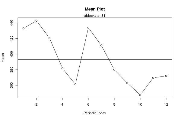
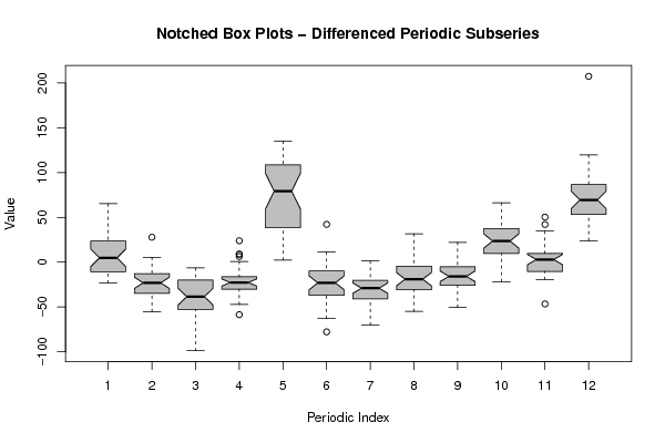
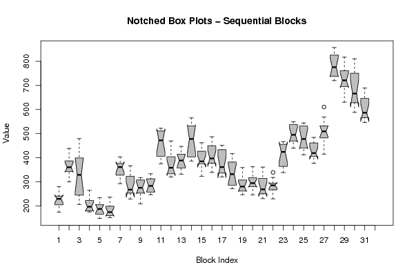
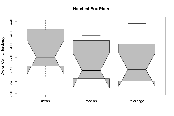
| Title produced by software | Mean Plot | ||||||||||||||||||||
| Date of computation | Fri, 23 Dec 2011 06:39:36 -0500 | ||||||||||||||||||||
| Cite this page as follows | Statistical Computations at FreeStatistics.org, Office for Research Development and Education, URL https://freestatistics.org/blog/index.php?v=date/2011/Dec/23/t1324640401260t4i1i62zqt1n.htm/, Retrieved Mon, 29 Apr 2024 18:51:25 +0000 | ||||||||||||||||||||
| Statistical Computations at FreeStatistics.org, Office for Research Development and Education, URL https://freestatistics.org/blog/index.php?pk=160300, Retrieved Mon, 29 Apr 2024 18:51:25 +0000 | |||||||||||||||||||||
| QR Codes: | |||||||||||||||||||||
|
| |||||||||||||||||||||
| Original text written by user: | |||||||||||||||||||||
| IsPrivate? | No (this computation is public) | ||||||||||||||||||||
| User-defined keywords | |||||||||||||||||||||
| Estimated Impact | 75 | ||||||||||||||||||||
Tree of Dependent Computations | |||||||||||||||||||||
| Family? (F = Feedback message, R = changed R code, M = changed R Module, P = changed Parameters, D = changed Data) | |||||||||||||||||||||
| - [Bivariate Data Series] [Bivariate dataset] [2008-01-05 23:51:08] [74be16979710d4c4e7c6647856088456] F RMPD [Mean Plot] [Colombia Coffee] [2008-01-07 13:38:24] [74be16979710d4c4e7c6647856088456] - RMPD [Mean Plot] [Workshop 6 - Assi...] [2011-11-14 13:16:48] [ec29c78521a0445a37e4526edb78f709] - D [Mean Plot] [Paper 3] [2011-12-23 11:39:36] [8829043a11b4adcf2fcb2d15cd36bb4f] [Current] | |||||||||||||||||||||
| Feedback Forum | |||||||||||||||||||||
Post a new message | |||||||||||||||||||||
Dataset | |||||||||||||||||||||
| Dataseries X: | |||||||||||||||||||||
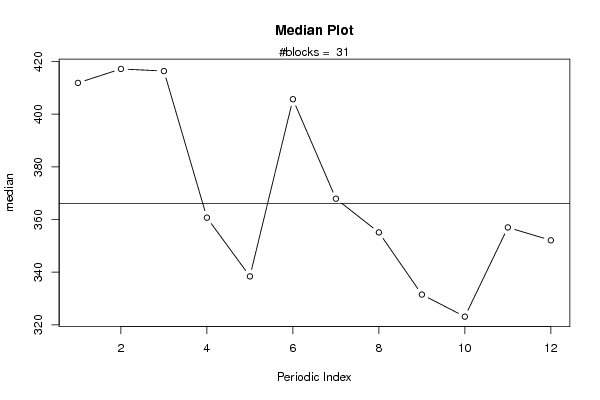
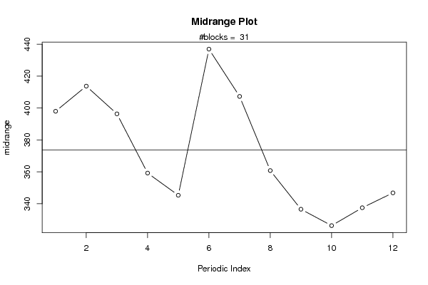
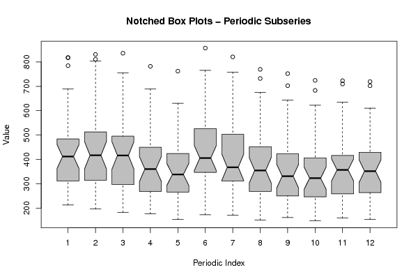
235.1 280.7 264.6 240.7 201.4 240.8 241.1 223.8 206.1 174.7 203.3 220.5 299.5 347.4 338.3 327.7 351.6 396.6 438.8 395.6 363.5 378.8 357 369 464.8 479.1 431.3 366.5 326.3 355.1 331.6 261.3 249 205.5 235.6 240.9 264.9 253.8 232.3 193.8 177 213.2 207.2 180.6 188.6 175.4 199 179.6 225.8 234 200.2 183.6 178.2 203.2 208.5 191.8 172.8 148 159.4 154.5 213.2 196.4 182.8 176.4 153.6 173.2 171 151.2 161.9 157.2 201.7 236.4 356.1 398.3 403.7 384.6 365.8 368.1 367.9 347 343.3 292.9 311.5 300.9 366.9 356.9 329.7 316.2 269 289.3 266.2 253.6 233.8 228.4 253.6 260.1 306.6 309.2 309.5 271 279.9 317.9 298.4 246.7 227.3 209.1 259.9 266 320.6 308.5 282.2 262.7 263.5 313.1 284.3 252.6 250.3 246.5 312.7 333.2 446.4 511.6 515.5 506.4 483.2 522.3 509.8 460.7 405.8 375 378.5 406.8 467.8 469.8 429.8 355.8 332.7 378 360.5 334.7 319.5 323.1 363.6 352.1 411.9 388.6 416.4 360.7 338 417.2 388.4 371.1 331.5 353.7 396.7 447 533.5 565.4 542.3 488.7 467.1 531.3 496.1 444 403.4 386.3 394.1 404.1 462.1 448.1 432.3 386.3 395.2 421.9 382.9 384.2 345.5 323.4 372.6 376 462.7 487 444.2 399.3 394.9 455.4 414 375.5 347 339.4 385.8 378.8 451.8 446.1 422.5 383.1 352.8 445.3 367.5 355.1 326.2 319.8 331.8 340.9 394.1 417.2 369.9 349.2 321.4 405.7 342.9 316.5 284.2 270.9 288.8 278.8 324.4 310.9 299 273 279.3 359.2 305 282.1 250.3 246.5 257.9 266.5 315.9 318.4 295.4 266.4 245.8 362.8 324.9 294.2 289.5 295.2 290.3 272 307.4 328.7 292.9 249.1 230.4 361.5 321.7 277.2 260.7 251 257.6 241.8 287.5 292.3 274.7 254.2 230 339 318.2 287 295.8 284 271 262.7 340.6 379.4 373.3 355.2 338.4 466.9 451 422 429.2 425.9 460.7 463.6 541.4 544.2 517.5 469.4 439.4 549 533 506.1 484 457 481.5 469.5 544.7 541.2 521.5 469.7 434.4 542.6 517.3 485.7 465.8 447 426.6 411.6 467.5 484.5 451.2 417.4 379.9 484.7 455 420.8 416.5 376.3 405.6 405.8 500.8 514 475.5 430.1 414.4 538 526 488.5 520.2 504.4 568.5 610.6 818 830.9 835.9 782 762.3 856.9 820.9 769.6 752.2 724.4 723.1 719.5 817.4 803.3 752.5 689 630.4 765.5 757.7 732.2 702.6 683.3 709.5 702.2 784.8 810.9 755.6 656.8 615.1 745.3 694.1 675.7 643.7 622.1 634.6 588 689.7 673.9 647.9 568.8 545.7 632.6 643.8 593.1 579.7 546 562.9 572.5 | |||||||||||||||||||||
Tables (Output of Computation) | |||||||||||||||||||||
| |||||||||||||||||||||
Figures (Output of Computation) | |||||||||||||||||||||
Input Parameters & R Code | |||||||||||||||||||||
| Parameters (Session): | |||||||||||||||||||||
| par1 = 12 ; | |||||||||||||||||||||
| Parameters (R input): | |||||||||||||||||||||
| par1 = 12 ; | |||||||||||||||||||||
| R code (references can be found in the software module): | |||||||||||||||||||||
par1 <- as.numeric(par1) | |||||||||||||||||||||