Repository of Reproducible Computations

Free Statistics

of Irreproducible Research!

Author's title

Author

*The author of this computation has been verified*

R Software Module

rwasp_autocorrelation.wasp

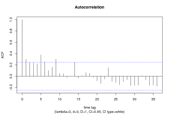
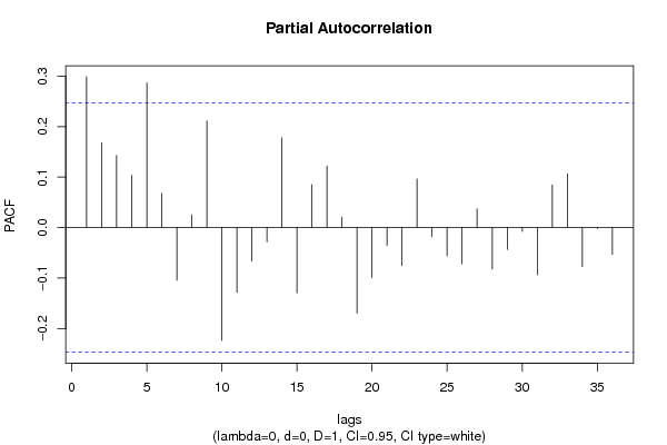
Title produced by software

(Partial) Autocorrelation Function

Date of computation

Fri, 23 Dec 2011 06:12:37 -0500

Cite this page as follows

Statistical Computations at FreeStatistics.org, Office for Research Development and Education, URL https://freestatistics.org/blog/index.php?v=date/2011/Dec/23/t13246387652mhh9ldtfncfx8n.htm/, Retrieved Mon, 29 Apr 2024 17:34:52 +0000

Statistical Computations at FreeStatistics.org, Office for Research Development and Education, URL https://freestatistics.org/blog/index.php?pk=160280, Retrieved Mon, 29 Apr 2024 17:34:52 +0000

QR Codes:

Paste this QR Code to cite your computation.

Original text written by user:

IsPrivate?

No (this computation is public)

User-defined keywords

Estimated Impact

111

Family? (F = Feedback message, R = changed R code, M = changed R Module, P = changed Parameters, D = changed Data)

-     [Univariate Explorative Data Analysis] [Run Sequence gebo...] [2008-12-12 13:32:37] [76963dc1903f0f612b6153510a3818cf]
- R  D  [Univariate Explorative Data Analysis] [Run Sequence gebo...] [2008-12-17 12:14:40] [76963dc1903f0f612b6153510a3818cf]
-         [Univariate Explorative Data Analysis] [Run Sequence Plot...] [2008-12-22 18:19:51] [1ce0d16c8f4225c977b42c8fa93bc163]
- RMP       [Univariate Data Series] [Identifying Integ...] [2009-11-22 12:08:06] [b98453cac15ba1066b407e146608df68]
- RMP         [(Partial) Autocorrelation Function] [] [2011-12-03 12:00:09] [84fecfa8c8107ac4e0024d8b1730a531]
- R             [(Partial) Autocorrelation Function] [] [2011-12-18 18:21:33] [74be16979710d4c4e7c6647856088456]
-                   [(Partial) Autocorrelation Function] [] [2011-12-23 11:12:37] [a23917169fba894c1fbb2182d294ed58] [Current]

Feedback Forum

Post a new message

Dataseries X:

Download CSV

Histogram

Boxplots

Summary of computational transaction
Raw Input	view raw input (R code)
Raw Output	view raw output of R engine
Computing time	2 seconds
R Server	'Herman Ole Andreas Wold' @ wold.wessa.net

\begin{tabular}{lllllllll}
\hline
Summary of computational transaction \tabularnewline
Raw Input & view raw input (R code)  \tabularnewline
Raw Output & view raw output of R engine  \tabularnewline
Computing time & 2 seconds \tabularnewline
R Server & 'Herman Ole Andreas Wold' @ wold.wessa.net \tabularnewline
\hline
\end{tabular}
%Source: https://freestatistics.org/blog/index.php?pk=160280&T=0

[TABLE]
[ROW][C]Summary of computational transaction[/C][/ROW]
[ROW][C]Raw Input[/C][C]view raw input (R code) [/C][/ROW]
[ROW][C]Raw Output[/C][C]view raw output of R engine [/C][/ROW]
[ROW][C]Computing time[/C][C]2 seconds[/C][/ROW]
[ROW][C]R Server[/C][C]'Herman Ole Andreas Wold' @ wold.wessa.net[/C][/ROW]
[/TABLE]
Source: https://freestatistics.org/blog/index.php?pk=160280&T=0

Globally Unique Identifier (entire table): ba.freestatistics.org/blog/index.php?pk=160280&T=0

As an alternative you can also use a QR Code:

The GUIDs for individual cells are displayed in the table below:

Summary of computational transaction
Raw Input	view raw input (R code)
Raw Output	view raw output of R engine
Computing time	2 seconds
R Server	'Herman Ole Andreas Wold' @ wold.wessa.net

Autocorrelation Function
Time lag k	ACF(k)	T-STAT	P-value
1	0.298808	2.3717	0.010387
2	0.242329	1.9234	0.029474
3	0.236977	1.8809	0.032301
4	0.218099	1.7311	0.044164
5	0.379693	3.0137	0.001857
6	0.256652	2.0371	0.022923
7	0.103456	0.8212	0.207327
8	0.16341	1.297	0.099675
9	0.301068	2.3897	0.009934
10	0.054693	0.4341	0.332845
11	0.045903	0.3643	0.35841
12	-0.022318	-0.1771	0.429981
13	-0.001837	-0.0146	0.494207
14	0.247977	1.9683	0.026722
15	-0.03128	-0.2483	0.402364
16	0.007348	0.0583	0.476838
17	0.066432	0.5273	0.299922
18	0.057292	0.4547	0.32543
19	-0.01855	-0.1472	0.441709
20	-0.082949	-0.6584	0.256344
21	-0.126996	-1.008	0.158654
22	-0.047601	-0.3778	0.353418
23	0.148519	1.1788	0.121449
24	-0.095645	-0.7592	0.225294
25	-0.114569	-0.9094	0.183313
26	-0.149371	-1.1856	0.120118
27	-0.095211	-0.7557	0.22632
28	-0.062579	-0.4967	0.310563
29	-0.167297	-1.3279	0.094505
30	-0.161989	-1.2857	0.101619
31	-0.158029	-1.2543	0.10718
32	0.009467	0.0751	0.470171
33	-0.064231	-0.5098	0.30598
34	-0.163128	-1.2948	0.10006
35	-0.158027	-1.2543	0.107184
36	-0.175246	-1.391	0.084564

\begin{tabular}{lllllllll}
\hline
Autocorrelation Function \tabularnewline
Time lag k & ACF(k) & T-STAT & P-value \tabularnewline
1 & 0.298808 & 2.3717 & 0.010387 \tabularnewline
2 & 0.242329 & 1.9234 & 0.029474 \tabularnewline
3 & 0.236977 & 1.8809 & 0.032301 \tabularnewline
4 & 0.218099 & 1.7311 & 0.044164 \tabularnewline
5 & 0.379693 & 3.0137 & 0.001857 \tabularnewline
6 & 0.256652 & 2.0371 & 0.022923 \tabularnewline
7 & 0.103456 & 0.8212 & 0.207327 \tabularnewline
8 & 0.16341 & 1.297 & 0.099675 \tabularnewline
9 & 0.301068 & 2.3897 & 0.009934 \tabularnewline
10 & 0.054693 & 0.4341 & 0.332845 \tabularnewline
11 & 0.045903 & 0.3643 & 0.35841 \tabularnewline
12 & -0.022318 & -0.1771 & 0.429981 \tabularnewline
13 & -0.001837 & -0.0146 & 0.494207 \tabularnewline
14 & 0.247977 & 1.9683 & 0.026722 \tabularnewline
15 & -0.03128 & -0.2483 & 0.402364 \tabularnewline
16 & 0.007348 & 0.0583 & 0.476838 \tabularnewline
17 & 0.066432 & 0.5273 & 0.299922 \tabularnewline
18 & 0.057292 & 0.4547 & 0.32543 \tabularnewline
19 & -0.01855 & -0.1472 & 0.441709 \tabularnewline
20 & -0.082949 & -0.6584 & 0.256344 \tabularnewline
21 & -0.126996 & -1.008 & 0.158654 \tabularnewline
22 & -0.047601 & -0.3778 & 0.353418 \tabularnewline
23 & 0.148519 & 1.1788 & 0.121449 \tabularnewline
24 & -0.095645 & -0.7592 & 0.225294 \tabularnewline
25 & -0.114569 & -0.9094 & 0.183313 \tabularnewline
26 & -0.149371 & -1.1856 & 0.120118 \tabularnewline
27 & -0.095211 & -0.7557 & 0.22632 \tabularnewline
28 & -0.062579 & -0.4967 & 0.310563 \tabularnewline
29 & -0.167297 & -1.3279 & 0.094505 \tabularnewline
30 & -0.161989 & -1.2857 & 0.101619 \tabularnewline
31 & -0.158029 & -1.2543 & 0.10718 \tabularnewline
32 & 0.009467 & 0.0751 & 0.470171 \tabularnewline
33 & -0.064231 & -0.5098 & 0.30598 \tabularnewline
34 & -0.163128 & -1.2948 & 0.10006 \tabularnewline
35 & -0.158027 & -1.2543 & 0.107184 \tabularnewline
36 & -0.175246 & -1.391 & 0.084564 \tabularnewline
\hline
\end{tabular}
%Source: https://freestatistics.org/blog/index.php?pk=160280&T=1

[TABLE]
[ROW][C]Autocorrelation Function[/C][/ROW]
[ROW][C]Time lag k[/C][C]ACF(k)[/C][C]T-STAT[/C][C]P-value[/C][/ROW]
[ROW][C]1[/C][C]0.298808[/C][C]2.3717[/C][C]0.010387[/C][/ROW]
[ROW][C]2[/C][C]0.242329[/C][C]1.9234[/C][C]0.029474[/C][/ROW]
[ROW][C]3[/C][C]0.236977[/C][C]1.8809[/C][C]0.032301[/C][/ROW]
[ROW][C]4[/C][C]0.218099[/C][C]1.7311[/C][C]0.044164[/C][/ROW]
[ROW][C]5[/C][C]0.379693[/C][C]3.0137[/C][C]0.001857[/C][/ROW]
[ROW][C]6[/C][C]0.256652[/C][C]2.0371[/C][C]0.022923[/C][/ROW]
[ROW][C]7[/C][C]0.103456[/C][C]0.8212[/C][C]0.207327[/C][/ROW]
[ROW][C]8[/C][C]0.16341[/C][C]1.297[/C][C]0.099675[/C][/ROW]
[ROW][C]9[/C][C]0.301068[/C][C]2.3897[/C][C]0.009934[/C][/ROW]
[ROW][C]10[/C][C]0.054693[/C][C]0.4341[/C][C]0.332845[/C][/ROW]
[ROW][C]11[/C][C]0.045903[/C][C]0.3643[/C][C]0.35841[/C][/ROW]
[ROW][C]12[/C][C]-0.022318[/C][C]-0.1771[/C][C]0.429981[/C][/ROW]
[ROW][C]13[/C][C]-0.001837[/C][C]-0.0146[/C][C]0.494207[/C][/ROW]
[ROW][C]14[/C][C]0.247977[/C][C]1.9683[/C][C]0.026722[/C][/ROW]
[ROW][C]15[/C][C]-0.03128[/C][C]-0.2483[/C][C]0.402364[/C][/ROW]
[ROW][C]16[/C][C]0.007348[/C][C]0.0583[/C][C]0.476838[/C][/ROW]
[ROW][C]17[/C][C]0.066432[/C][C]0.5273[/C][C]0.299922[/C][/ROW]
[ROW][C]18[/C][C]0.057292[/C][C]0.4547[/C][C]0.32543[/C][/ROW]
[ROW][C]19[/C][C]-0.01855[/C][C]-0.1472[/C][C]0.441709[/C][/ROW]
[ROW][C]20[/C][C]-0.082949[/C][C]-0.6584[/C][C]0.256344[/C][/ROW]
[ROW][C]21[/C][C]-0.126996[/C][C]-1.008[/C][C]0.158654[/C][/ROW]
[ROW][C]22[/C][C]-0.047601[/C][C]-0.3778[/C][C]0.353418[/C][/ROW]
[ROW][C]23[/C][C]0.148519[/C][C]1.1788[/C][C]0.121449[/C][/ROW]
[ROW][C]24[/C][C]-0.095645[/C][C]-0.7592[/C][C]0.225294[/C][/ROW]
[ROW][C]25[/C][C]-0.114569[/C][C]-0.9094[/C][C]0.183313[/C][/ROW]
[ROW][C]26[/C][C]-0.149371[/C][C]-1.1856[/C][C]0.120118[/C][/ROW]
[ROW][C]27[/C][C]-0.095211[/C][C]-0.7557[/C][C]0.22632[/C][/ROW]
[ROW][C]28[/C][C]-0.062579[/C][C]-0.4967[/C][C]0.310563[/C][/ROW]
[ROW][C]29[/C][C]-0.167297[/C][C]-1.3279[/C][C]0.094505[/C][/ROW]
[ROW][C]30[/C][C]-0.161989[/C][C]-1.2857[/C][C]0.101619[/C][/ROW]
[ROW][C]31[/C][C]-0.158029[/C][C]-1.2543[/C][C]0.10718[/C][/ROW]
[ROW][C]32[/C][C]0.009467[/C][C]0.0751[/C][C]0.470171[/C][/ROW]
[ROW][C]33[/C][C]-0.064231[/C][C]-0.5098[/C][C]0.30598[/C][/ROW]
[ROW][C]34[/C][C]-0.163128[/C][C]-1.2948[/C][C]0.10006[/C][/ROW]
[ROW][C]35[/C][C]-0.158027[/C][C]-1.2543[/C][C]0.107184[/C][/ROW]
[ROW][C]36[/C][C]-0.175246[/C][C]-1.391[/C][C]0.084564[/C][/ROW]
[/TABLE]
Source: https://freestatistics.org/blog/index.php?pk=160280&T=1

Globally Unique Identifier (entire table): ba.freestatistics.org/blog/index.php?pk=160280&T=1

As an alternative you can also use a QR Code:

The GUIDs for individual cells are displayed in the table below:

Autocorrelation Function
Time lag k	ACF(k)	T-STAT	P-value
1	0.298808	2.3717	0.010387
2	0.242329	1.9234	0.029474
3	0.236977	1.8809	0.032301
4	0.218099	1.7311	0.044164
5	0.379693	3.0137	0.001857
6	0.256652	2.0371	0.022923
7	0.103456	0.8212	0.207327
8	0.16341	1.297	0.099675
9	0.301068	2.3897	0.009934
10	0.054693	0.4341	0.332845
11	0.045903	0.3643	0.35841
12	-0.022318	-0.1771	0.429981
13	-0.001837	-0.0146	0.494207
14	0.247977	1.9683	0.026722
15	-0.03128	-0.2483	0.402364
16	0.007348	0.0583	0.476838
17	0.066432	0.5273	0.299922
18	0.057292	0.4547	0.32543
19	-0.01855	-0.1472	0.441709
20	-0.082949	-0.6584	0.256344
21	-0.126996	-1.008	0.158654
22	-0.047601	-0.3778	0.353418
23	0.148519	1.1788	0.121449
24	-0.095645	-0.7592	0.225294
25	-0.114569	-0.9094	0.183313
26	-0.149371	-1.1856	0.120118
27	-0.095211	-0.7557	0.22632
28	-0.062579	-0.4967	0.310563
29	-0.167297	-1.3279	0.094505
30	-0.161989	-1.2857	0.101619
31	-0.158029	-1.2543	0.10718
32	0.009467	0.0751	0.470171
33	-0.064231	-0.5098	0.30598
34	-0.163128	-1.2948	0.10006
35	-0.158027	-1.2543	0.107184
36	-0.175246	-1.391	0.084564

Partial Autocorrelation Function
Time lag k	PACF(k)	T-STAT	P-value
1	0.298808	2.3717	0.010387
2	0.168047	1.3338	0.09353
3	0.142963	1.1347	0.130393
4	0.103878	0.8245	0.206382
5	0.28661	2.2749	0.013163
6	0.06781	0.5382	0.296158
7	-0.104479	-0.8293	0.205041
8	0.025232	0.2003	0.420955
9	0.21101	1.6748	0.049462
10	-0.223667	-1.7753	0.040339
11	-0.128247	-1.0179	0.156302
12	-0.066198	-0.5254	0.300564
13	-0.02781	-0.2207	0.413007
14	0.177805	1.4113	0.08154
15	-0.129422	-1.0273	0.154115
16	0.085174	0.676	0.250742
17	0.12159	0.9651	0.169095
18	0.020396	0.1619	0.435957
19	-0.169491	-1.3453	0.091677
20	-0.098734	-0.7837	0.218084
21	-0.035407	-0.281	0.389803
22	-0.075139	-0.5964	0.276523
23	0.096365	0.7649	0.223601
24	-0.018127	-0.1439	0.443027
25	-0.055942	-0.444	0.329272
26	-0.071761	-0.5696	0.285492
27	0.036998	0.2937	0.38499
28	-0.082299	-0.6532	0.257993
29	-0.043481	-0.3451	0.365577
30	-0.007729	-0.0614	0.475637
31	-0.093437	-0.7416	0.230533
32	0.084525	0.6709	0.252371
33	0.106658	0.8466	0.200219
34	-0.077354	-0.614	0.270721
35	-0.002124	-0.0169	0.4933
36	-0.053348	-0.4234	0.336709

\begin{tabular}{lllllllll}
\hline
Partial Autocorrelation Function \tabularnewline
Time lag k & PACF(k) & T-STAT & P-value \tabularnewline
1 & 0.298808 & 2.3717 & 0.010387 \tabularnewline
2 & 0.168047 & 1.3338 & 0.09353 \tabularnewline
3 & 0.142963 & 1.1347 & 0.130393 \tabularnewline
4 & 0.103878 & 0.8245 & 0.206382 \tabularnewline
5 & 0.28661 & 2.2749 & 0.013163 \tabularnewline
6 & 0.06781 & 0.5382 & 0.296158 \tabularnewline
7 & -0.104479 & -0.8293 & 0.205041 \tabularnewline
8 & 0.025232 & 0.2003 & 0.420955 \tabularnewline
9 & 0.21101 & 1.6748 & 0.049462 \tabularnewline
10 & -0.223667 & -1.7753 & 0.040339 \tabularnewline
11 & -0.128247 & -1.0179 & 0.156302 \tabularnewline
12 & -0.066198 & -0.5254 & 0.300564 \tabularnewline
13 & -0.02781 & -0.2207 & 0.413007 \tabularnewline
14 & 0.177805 & 1.4113 & 0.08154 \tabularnewline
15 & -0.129422 & -1.0273 & 0.154115 \tabularnewline
16 & 0.085174 & 0.676 & 0.250742 \tabularnewline
17 & 0.12159 & 0.9651 & 0.169095 \tabularnewline
18 & 0.020396 & 0.1619 & 0.435957 \tabularnewline
19 & -0.169491 & -1.3453 & 0.091677 \tabularnewline
20 & -0.098734 & -0.7837 & 0.218084 \tabularnewline
21 & -0.035407 & -0.281 & 0.389803 \tabularnewline
22 & -0.075139 & -0.5964 & 0.276523 \tabularnewline
23 & 0.096365 & 0.7649 & 0.223601 \tabularnewline
24 & -0.018127 & -0.1439 & 0.443027 \tabularnewline
25 & -0.055942 & -0.444 & 0.329272 \tabularnewline
26 & -0.071761 & -0.5696 & 0.285492 \tabularnewline
27 & 0.036998 & 0.2937 & 0.38499 \tabularnewline
28 & -0.082299 & -0.6532 & 0.257993 \tabularnewline
29 & -0.043481 & -0.3451 & 0.365577 \tabularnewline
30 & -0.007729 & -0.0614 & 0.475637 \tabularnewline
31 & -0.093437 & -0.7416 & 0.230533 \tabularnewline
32 & 0.084525 & 0.6709 & 0.252371 \tabularnewline
33 & 0.106658 & 0.8466 & 0.200219 \tabularnewline
34 & -0.077354 & -0.614 & 0.270721 \tabularnewline
35 & -0.002124 & -0.0169 & 0.4933 \tabularnewline
36 & -0.053348 & -0.4234 & 0.336709 \tabularnewline
\hline
\end{tabular}
%Source: https://freestatistics.org/blog/index.php?pk=160280&T=2

[TABLE]
[ROW][C]Partial Autocorrelation Function[/C][/ROW]
[ROW][C]Time lag k[/C][C]PACF(k)[/C][C]T-STAT[/C][C]P-value[/C][/ROW]
[ROW][C]1[/C][C]0.298808[/C][C]2.3717[/C][C]0.010387[/C][/ROW]
[ROW][C]2[/C][C]0.168047[/C][C]1.3338[/C][C]0.09353[/C][/ROW]
[ROW][C]3[/C][C]0.142963[/C][C]1.1347[/C][C]0.130393[/C][/ROW]
[ROW][C]4[/C][C]0.103878[/C][C]0.8245[/C][C]0.206382[/C][/ROW]
[ROW][C]5[/C][C]0.28661[/C][C]2.2749[/C][C]0.013163[/C][/ROW]
[ROW][C]6[/C][C]0.06781[/C][C]0.5382[/C][C]0.296158[/C][/ROW]
[ROW][C]7[/C][C]-0.104479[/C][C]-0.8293[/C][C]0.205041[/C][/ROW]
[ROW][C]8[/C][C]0.025232[/C][C]0.2003[/C][C]0.420955[/C][/ROW]
[ROW][C]9[/C][C]0.21101[/C][C]1.6748[/C][C]0.049462[/C][/ROW]
[ROW][C]10[/C][C]-0.223667[/C][C]-1.7753[/C][C]0.040339[/C][/ROW]
[ROW][C]11[/C][C]-0.128247[/C][C]-1.0179[/C][C]0.156302[/C][/ROW]
[ROW][C]12[/C][C]-0.066198[/C][C]-0.5254[/C][C]0.300564[/C][/ROW]
[ROW][C]13[/C][C]-0.02781[/C][C]-0.2207[/C][C]0.413007[/C][/ROW]
[ROW][C]14[/C][C]0.177805[/C][C]1.4113[/C][C]0.08154[/C][/ROW]
[ROW][C]15[/C][C]-0.129422[/C][C]-1.0273[/C][C]0.154115[/C][/ROW]
[ROW][C]16[/C][C]0.085174[/C][C]0.676[/C][C]0.250742[/C][/ROW]
[ROW][C]17[/C][C]0.12159[/C][C]0.9651[/C][C]0.169095[/C][/ROW]
[ROW][C]18[/C][C]0.020396[/C][C]0.1619[/C][C]0.435957[/C][/ROW]
[ROW][C]19[/C][C]-0.169491[/C][C]-1.3453[/C][C]0.091677[/C][/ROW]
[ROW][C]20[/C][C]-0.098734[/C][C]-0.7837[/C][C]0.218084[/C][/ROW]
[ROW][C]21[/C][C]-0.035407[/C][C]-0.281[/C][C]0.389803[/C][/ROW]
[ROW][C]22[/C][C]-0.075139[/C][C]-0.5964[/C][C]0.276523[/C][/ROW]
[ROW][C]23[/C][C]0.096365[/C][C]0.7649[/C][C]0.223601[/C][/ROW]
[ROW][C]24[/C][C]-0.018127[/C][C]-0.1439[/C][C]0.443027[/C][/ROW]
[ROW][C]25[/C][C]-0.055942[/C][C]-0.444[/C][C]0.329272[/C][/ROW]
[ROW][C]26[/C][C]-0.071761[/C][C]-0.5696[/C][C]0.285492[/C][/ROW]
[ROW][C]27[/C][C]0.036998[/C][C]0.2937[/C][C]0.38499[/C][/ROW]
[ROW][C]28[/C][C]-0.082299[/C][C]-0.6532[/C][C]0.257993[/C][/ROW]
[ROW][C]29[/C][C]-0.043481[/C][C]-0.3451[/C][C]0.365577[/C][/ROW]
[ROW][C]30[/C][C]-0.007729[/C][C]-0.0614[/C][C]0.475637[/C][/ROW]
[ROW][C]31[/C][C]-0.093437[/C][C]-0.7416[/C][C]0.230533[/C][/ROW]
[ROW][C]32[/C][C]0.084525[/C][C]0.6709[/C][C]0.252371[/C][/ROW]
[ROW][C]33[/C][C]0.106658[/C][C]0.8466[/C][C]0.200219[/C][/ROW]
[ROW][C]34[/C][C]-0.077354[/C][C]-0.614[/C][C]0.270721[/C][/ROW]
[ROW][C]35[/C][C]-0.002124[/C][C]-0.0169[/C][C]0.4933[/C][/ROW]
[ROW][C]36[/C][C]-0.053348[/C][C]-0.4234[/C][C]0.336709[/C][/ROW]
[/TABLE]
Source: https://freestatistics.org/blog/index.php?pk=160280&T=2

Globally Unique Identifier (entire table): ba.freestatistics.org/blog/index.php?pk=160280&T=2

As an alternative you can also use a QR Code:

The GUIDs for individual cells are displayed in the table below:

Partial Autocorrelation Function
Time lag k	PACF(k)	T-STAT	P-value
1	0.298808	2.3717	0.010387
2	0.168047	1.3338	0.09353
3	0.142963	1.1347	0.130393
4	0.103878	0.8245	0.206382
5	0.28661	2.2749	0.013163
6	0.06781	0.5382	0.296158
7	-0.104479	-0.8293	0.205041
8	0.025232	0.2003	0.420955
9	0.21101	1.6748	0.049462
10	-0.223667	-1.7753	0.040339
11	-0.128247	-1.0179	0.156302
12	-0.066198	-0.5254	0.300564
13	-0.02781	-0.2207	0.413007
14	0.177805	1.4113	0.08154
15	-0.129422	-1.0273	0.154115
16	0.085174	0.676	0.250742
17	0.12159	0.9651	0.169095
18	0.020396	0.1619	0.435957
19	-0.169491	-1.3453	0.091677
20	-0.098734	-0.7837	0.218084
21	-0.035407	-0.281	0.389803
22	-0.075139	-0.5964	0.276523
23	0.096365	0.7649	0.223601
24	-0.018127	-0.1439	0.443027
25	-0.055942	-0.444	0.329272
26	-0.071761	-0.5696	0.285492
27	0.036998	0.2937	0.38499
28	-0.082299	-0.6532	0.257993
29	-0.043481	-0.3451	0.365577
30	-0.007729	-0.0614	0.475637
31	-0.093437	-0.7416	0.230533
32	0.084525	0.6709	0.252371
33	0.106658	0.8466	0.200219
34	-0.077354	-0.614	0.270721
35	-0.002124	-0.0169	0.4933
36	-0.053348	-0.4234	0.336709

Figure 1

PNG link

Postscript link

PDF link

Figure 2

PNG link

Postscript link

PDF link

Figure 3

PNG link

Postscript link

PDF link

Parameters (Session):

par1 = 36 ; par2 = 0.0 ; par3 = 0 ; par4 = 1 ; par5 = 12 ; par6 = White Noise ; par7 = 0.95 ;

Parameters (R input):

par1 = 36 ; par2 = 0.0 ; par3 = 0 ; par4 = 1 ; par5 = 12 ; par6 = White Noise ; par7 = 0.95 ; par8 = ;

R code (references can be found in the software module):

if (par1 == 'Default') {
par1 = 10*log10(length(x))
} else {
par1 <- as.numeric(par1)
}
par2 <- as.numeric(par2)
par3 <- as.numeric(par3)
par4 <- as.numeric(par4)
par5 <- as.numeric(par5)
if (par6 == 'White Noise') par6 <- 'white' else par6 <- 'ma'
par7 <- as.numeric(par7)
if (par8 != '') par8 <- as.numeric(par8)
ox <- x
if (par8 == '') {
if (par2 == 0) {
x <- log(x)
} else {
x <- (x ^ par2 - 1) / par2
}
} else {
x <- log(x,base=par8)
}
if (par3 > 0) x <- diff(x,lag=1,difference=par3)
if (par4 > 0) x <- diff(x,lag=par5,difference=par4)
bitmap(file='picts.png')
op <- par(mfrow=c(2,1))
plot(ox,type='l',main='Original Time Series',xlab='time',ylab='value')
if (par8=='') {
mytitle <- paste('Working Time Series (lambda=',par2,', d=',par3,', D=',par4,')',sep='')
mysub <- paste('(lambda=',par2,', d=',par3,', D=',par4,', CI=', par7, ', CI type=',par6,')',sep='')
} else {
mytitle <- paste('Working Time Series (base=',par8,', d=',par3,', D=',par4,')',sep='')
mysub <- paste('(base=',par8,', d=',par3,', D=',par4,', CI=', par7, ', CI type=',par6,')',sep='')
}
plot(x,type='l', main=mytitle,xlab='time',ylab='value')
par(op)
dev.off()
bitmap(file='pic1.png')
racf <- acf(x, par1, main='Autocorrelation', xlab='time lag', ylab='ACF', ci.type=par6, ci=par7, sub=mysub)
dev.off()
bitmap(file='pic2.png')
rpacf <- pacf(x,par1,main='Partial Autocorrelation',xlab='lags',ylab='PACF',sub=mysub)
dev.off()
(myacf <- c(racf$acf))
(mypacf <- c(rpacf$acf))
lengthx <- length(x)
sqrtn <- sqrt(lengthx)
load(file='createtable')
a<-table.start()
a<-table.row.start(a)
a<-table.element(a,'Autocorrelation Function',4,TRUE)
a<-table.row.end(a)
a<-table.row.start(a)
a<-table.element(a,'Time lag k',header=TRUE)
a<-table.element(a,hyperlink('basics.htm','ACF(k)','click here for more information about the Autocorrelation Function'),header=TRUE)
a<-table.element(a,'T-STAT',header=TRUE)
a<-table.element(a,'P-value',header=TRUE)
a<-table.row.end(a)
for (i in 2:(par1+1)) {
a<-table.row.start(a)
a<-table.element(a,i-1,header=TRUE)
a<-table.element(a,round(myacf[i],6))
mytstat <- myacf[i]*sqrtn
a<-table.element(a,round(mytstat,4))
a<-table.element(a,round(1-pt(abs(mytstat),lengthx),6))
a<-table.row.end(a)
}
a<-table.end(a)
table.save(a,file='mytable.tab')
a<-table.start()
a<-table.row.start(a)
a<-table.element(a,'Partial Autocorrelation Function',4,TRUE)
a<-table.row.end(a)
a<-table.row.start(a)
a<-table.element(a,'Time lag k',header=TRUE)
a<-table.element(a,hyperlink('basics.htm','PACF(k)','click here for more information about the Partial Autocorrelation Function'),header=TRUE)
a<-table.element(a,'T-STAT',header=TRUE)
a<-table.element(a,'P-value',header=TRUE)
a<-table.row.end(a)
for (i in 1:par1) {
a<-table.row.start(a)
a<-table.element(a,i,header=TRUE)
a<-table.element(a,round(mypacf[i],6))
mytstat <- mypacf[i]*sqrtn
a<-table.element(a,round(mytstat,4))
a<-table.element(a,round(1-pt(abs(mytstat),lengthx),6))
a<-table.row.end(a)
}
a<-table.end(a)
table.save(a,file='mytable1.tab')

Free Statistics

Description of Statistical Computation

Tree of Dependent Computations

Dataset

Tables (Output of Computation)

Figures (Output of Computation)

Input Parameters & R Code