Repository of Reproducible Computations

Free Statistics

of Irreproducible Research!

Author's title

Author

*The author of this computation has been verified*

R Software Module

rwasp_pairs.wasp

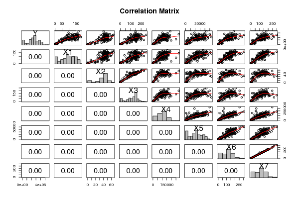
Title produced by software

Kendall tau Correlation Matrix

Date of computation

Fri, 23 Dec 2011 05:06:23 -0500

Cite this page as follows

Statistical Computations at FreeStatistics.org, Office for Research Development and Education, URL https://freestatistics.org/blog/index.php?v=date/2011/Dec/23/t132463491567wscnp9gkjjshr.htm/, Retrieved Mon, 29 Apr 2024 18:37:17 +0000

Statistical Computations at FreeStatistics.org, Office for Research Development and Education, URL https://freestatistics.org/blog/index.php?pk=160227, Retrieved Mon, 29 Apr 2024 18:37:17 +0000

QR Codes:

Paste this QR Code to cite your computation.

Original text written by user:

IsPrivate?

No (this computation is public)

User-defined keywords

Estimated Impact

183

Family? (F = Feedback message, R = changed R code, M = changed R Module, P = changed Parameters, D = changed Data)

-     [Kendall tau Correlation Matrix] [WS10] [2011-12-09 08:45:50] [09e53a95f5780167f20e6b4304200573]
- R     [Kendall tau Correlation Matrix] [WS 10 - Hall of fame] [2011-12-13 11:12:25] [c6dda33d269efe9a48a310f0c0798534]
-    D      [Kendall tau Correlation Matrix] [] [2011-12-23 10:06:23] [5fd8c857995b7937a45335fd5ccccdde] [Current]
-   P         [Kendall tau Correlation Matrix] [] [2011-12-23 10:09:18] [9b13650c94c5192ca5135ec8a1fa39f7] 

Feedback Forum

Post a new message

Dataseries X:

Download CSV

Histogram

Boxplots

279055	96	42	130	140824	32033	165	165
209884	75	38	143	110459	20654	135	132
233432	70	46	118	105079	16346	121	121
222117	134	42	146	112098	35926	148	145
179751	72	30	73	43929	10621	73	71
70849	8	35	89	76173	10024	49	47
568125	169	40	146	187326	43068	185	177
33186	1	18	22	22807	1271	5	5
227332	88	38	132	144408	34416	125	124
258676	98	37	92	66485	20318	93	92
341549	101	46	147	79089	24409	154	149
260484	122	60	203	81625	20648	98	93
202918	57	37	113	68788	12347	70	70
367799	139	55	171	103297	21857	148	148
269455	87	44	87	69446	11034	100	100
394578	176	63	208	114948	33433	150	142
335567	114	40	153	167949	35902	197	194
423110	121	43	97	125081	22355	114	113
182016	103	32	95	125818	31219	169	162
267365	135	52	197	136588	21983	200	186
279428	123	49	160	112431	40085	148	147
506616	97	41	148	103037	18507	140	137
201993	74	25	84	82317	16278	74	71
200004	103	57	227	118906	24662	128	123
257139	158	45	154	83515	31452	140	134
256931	113	42	151	104581	32580	116	115
296850	102	45	142	103129	22883	147	138
307100	132	43	148	83243	27652	132	125
184160	62	36	110	37110	9845	70	66
393860	150	45	149	113344	20190	144	137
309877	138	50	179	139165	46201	155	152
252512	50	50	149	86652	10971	165	159
367819	141	51	187	112302	34811	161	159
115602	48	42	153	69652	3029	31	31
430118	141	44	163	119442	38941	199	185
273950	83	42	127	69867	4958	78	78
428028	112	44	151	101629	32344	121	117
251306	79	40	100	70168	19433	112	109
115658	33	17	46	31081	12558	41	41
388812	149	43	156	103925	36524	158	149
343783	126	41	128	92622	26041	123	123
198635	81	41	111	79011	16637	104	103
213258	84	40	119	93487	28395	94	87
182398	68	49	148	64520	16747	73	71
157164	50	52	65	93473	9105	52	51
459440	101	42	134	114360	11941	71	70
78800	20	26	66	33032	7935	21	21
217575	101	59	201	96125	19499	155	155
368086	150	50	177	151911	22938	174	172
206448	115	50	156	89256	25314	136	133
244640	99	47	158	95676	28527	128	125
24188	8	4	7	5950	2694	7	7
399093	88	51	175	149695	20867	165	158
65029	21	18	61	32551	3597	21	21
101097	30	14	41	31701	5296	35	35
297973	97	41	133	100087	32982	137	133
369627	163	61	228	169707	38975	174	169
367127	132	40	140	150491	42721	257	256
374143	161	44	155	120192	41455	207	190
270099	89	40	141	95893	23923	103	100
391871	160	51	181	151715	26719	171	171
315924	139	29	75	176225	53405	279	267
291391	104	43	97	59900	12526	83	80
286417	100	42	142	104767	26584	130	126
270324	66	41	136	114799	37062	131	132
267432	163	30	87	72128	25696	126	121
215924	93	39	140	143592	24634	158	156
249232	85	51	169	89626	27269	138	133
260919	150	40	129	131072	25270	200	199
182961	143	29	92	126817	24634	104	98
256967	107	47	160	81351	17828	111	109
73566	22	23	67	22618	3007	26	25
272362	85	48	179	88977	20065	115	113
216802	86	38	90	92059	24648	127	126
228835	131	42	144	81897	21588	140	137
371391	140	46	144	108146	25217	121	121
392330	156	40	144	126372	30927	183	178
220401	81	45	134	249771	18487	68	63
225825	137	42	146	71154	18050	112	109
217623	102	41	121	71571	17696	103	101
199011	72	37	112	55918	17326	63	61
483074	161	47	145	160141	39361	166	157
145943	30	26	99	38692	9648	38	38
295224	120	48	96	102812	26759	163	159
80953	49	8	27	56622	7905	59	58
171206	63	27	77	15986	4527	27	27
179344	76	38	137	123534	41517	108	108
415550	85	41	151	108535	21261	88	83
366035	146	61	126	93879	36099	92	88
180679	165	45	159	144551	39039	170	164
298696	89	41	101	56750	13841	98	96
292260	168	42	144	127654	23841	205	192
199481	48	35	102	65594	8589	96	94
282361	149	36	135	59938	15049	107	107
329281	75	40	147	146975	39038	150	144
230588	103	40	155	165904	36774	138	136
297995	116	38	138	169265	40076	177	171
305984	165	43	113	183500	43840	213	210
416463	155	65	248	165986	43146	208	193
412530	165	33	116	184923	50099	307	297
297080	121	51	176	140358	40312	125	125
318283	156	45	140	149959	32616	208	204
202726	81	36	59	57224	11338	73	70
43287	13	19	64	43750	7409	49	49
223456	113	25	40	48029	18213	82	82
258249	112	44	98	104978	45873	206	205
299566	133	45	139	100046	39844	112	111
321797	169	44	135	101047	28317	139	135
170299	28	35	97	197426	24797	60	59
169545	121	46	142	160902	7471	70	70
354041	82	44	155	147172	27259	112	108
303273	148	45	115	109432	23201	142	141
23623	12	1	0	1168	238	11	11
195880	146	40	103	83248	28830	130	130
61857	23	11	30	25162	3913	31	28
207339	84	51	130	45724	9935	132	101
431443	163	38	102	110529	27738	219	216
21054	4	0	0	855	338	4	4
252805	81	30	77	101382	13326	102	97
31961	18	8	9	14116	3988	39	39
354622	118	43	150	89506	24347	125	119
251240	76	48	163	135356	27111	121	118
187003	55	49	148	116066	3938	42	41
172481	57	32	94	144244	17416	111	107
38214	16	8	21	8773	1888	16	16
256082	93	43	151	102153	18700	70	69
358276	137	52	187	117440	36809	162	160
211775	50	53	171	104128	24959	173	158
445926	152	49	170	134238	37343	171	161
348017	163	48	145	134047	21849	172	165
441946	142	56	198	279488	49809	254	246
208962	77	45	152	79756	21654	90	89
105332	42	40	112	66089	8728	50	49
315219	94	48	173	102070	20920	113	107
460249	126	50	177	146760	27195	187	182
160740	63	43	153	154771	1037	16	16
412099	127	46	161	165933	42570	175	173
173747	59	40	115	64593	17672	90	90
284582	117	45	147	92280	34245	140	140
283913	110	46	124	67150	16786	145	142
234262	44	37	57	128692	20954	141	126
386740	95	45	144	124089	16378	125	123
246963	128	39	126	125386	31852	241	239
173260	41	21	78	37238	2805	16	15
346748	146	50	153	140015	38086	175	170
176654	147	55	196	150047	21166	132	123
264767	121	40	130	154451	34672	154	151
314070	185	48	159	156349	36171	198	194
1	0	0	0	0	0	0	0
14688	4	0	0	6023	2065	5	5
98	0	0	0	0	0	0	0
455	0	0	0	0	0	0	0
0	0	0	0	0	0	0	0
0	0	0	0	0	0	0	0
284420	85	46	94	84601	19354	125	122
410509	157	52	129	68946	22124	174	173
0	0	0	0	0	0	0	0
203	0	0	0	0	0	0	0
7199	7	0	0	1644	556	6	6
46660	12	5	13	6179	2089	13	13
17547	0	1	4	3926	2658	3	3
121550	37	48	89	52789	1813	35	35
969	0	0	0	0	0	0	0
242258	62	34	71	100350	17372	80	72

Summary of computational transaction
Raw Input	view raw input (R code)
Raw Output	view raw output of R engine
Computing time	2 seconds
R Server	'Gwilym Jenkins' @ jenkins.wessa.net

\begin{tabular}{lllllllll}
\hline
Summary of computational transaction \tabularnewline
Raw Input & view raw input (R code)  \tabularnewline
Raw Output & view raw output of R engine  \tabularnewline
Computing time & 2 seconds \tabularnewline
R Server & 'Gwilym Jenkins' @ jenkins.wessa.net \tabularnewline
\hline
\end{tabular}
%Source: https://freestatistics.org/blog/index.php?pk=160227&T=0

[TABLE]
[ROW][C]Summary of computational transaction[/C][/ROW]
[ROW][C]Raw Input[/C][C]view raw input (R code) [/C][/ROW]
[ROW][C]Raw Output[/C][C]view raw output of R engine [/C][/ROW]
[ROW][C]Computing time[/C][C]2 seconds[/C][/ROW]
[ROW][C]R Server[/C][C]'Gwilym Jenkins' @ jenkins.wessa.net[/C][/ROW]
[/TABLE]
Source: https://freestatistics.org/blog/index.php?pk=160227&T=0

Globally Unique Identifier (entire table): ba.freestatistics.org/blog/index.php?pk=160227&T=0

As an alternative you can also use a QR Code:

The GUIDs for individual cells are displayed in the table below:

Summary of computational transaction
Raw Input	view raw input (R code)
Raw Output	view raw output of R engine
Computing time	2 seconds
R Server	'Gwilym Jenkins' @ jenkins.wessa.net

Correlations for all pairs of data series (method=pearson)
	Y	X1	X2	X3	X4	X5	X6	X7
Y	1	0.822	0.751	0.741	0.706	0.731	0.781	0.78
X1	0.822	1	0.732	0.732	0.685	0.781	0.83	0.831
X2	0.751	0.732	1	0.919	0.693	0.625	0.674	0.671
X3	0.741	0.732	0.919	1	0.72	0.664	0.685	0.682
X4	0.706	0.685	0.693	0.72	1	0.773	0.764	0.764
X5	0.731	0.781	0.625	0.664	0.773	1	0.859	0.861
X6	0.781	0.83	0.674	0.685	0.764	0.859	1	0.998
X7	0.78	0.831	0.671	0.682	0.764	0.861	0.998	1

\begin{tabular}{lllllllll}
\hline
Correlations for all pairs of data series (method=pearson) \tabularnewline
  & Y & X1 & X2 & X3 & X4 & X5 & X6 & X7 \tabularnewline
Y & 1 & 0.822 & 0.751 & 0.741 & 0.706 & 0.731 & 0.781 & 0.78 \tabularnewline
X1 & 0.822 & 1 & 0.732 & 0.732 & 0.685 & 0.781 & 0.83 & 0.831 \tabularnewline
X2 & 0.751 & 0.732 & 1 & 0.919 & 0.693 & 0.625 & 0.674 & 0.671 \tabularnewline
X3 & 0.741 & 0.732 & 0.919 & 1 & 0.72 & 0.664 & 0.685 & 0.682 \tabularnewline
X4 & 0.706 & 0.685 & 0.693 & 0.72 & 1 & 0.773 & 0.764 & 0.764 \tabularnewline
X5 & 0.731 & 0.781 & 0.625 & 0.664 & 0.773 & 1 & 0.859 & 0.861 \tabularnewline
X6 & 0.781 & 0.83 & 0.674 & 0.685 & 0.764 & 0.859 & 1 & 0.998 \tabularnewline
X7 & 0.78 & 0.831 & 0.671 & 0.682 & 0.764 & 0.861 & 0.998 & 1 \tabularnewline
\hline
\end{tabular}
%Source: https://freestatistics.org/blog/index.php?pk=160227&T=1

[TABLE]
[ROW][C]Correlations for all pairs of data series (method=pearson)[/C][/ROW]
[ROW][C] [/C][C]Y[/C][C]X1[/C][C]X2[/C][C]X3[/C][C]X4[/C][C]X5[/C][C]X6[/C][C]X7[/C][/ROW]
[ROW][C]Y[/C][C]1[/C][C]0.822[/C][C]0.751[/C][C]0.741[/C][C]0.706[/C][C]0.731[/C][C]0.781[/C][C]0.78[/C][/ROW]
[ROW][C]X1[/C][C]0.822[/C][C]1[/C][C]0.732[/C][C]0.732[/C][C]0.685[/C][C]0.781[/C][C]0.83[/C][C]0.831[/C][/ROW]
[ROW][C]X2[/C][C]0.751[/C][C]0.732[/C][C]1[/C][C]0.919[/C][C]0.693[/C][C]0.625[/C][C]0.674[/C][C]0.671[/C][/ROW]
[ROW][C]X3[/C][C]0.741[/C][C]0.732[/C][C]0.919[/C][C]1[/C][C]0.72[/C][C]0.664[/C][C]0.685[/C][C]0.682[/C][/ROW]
[ROW][C]X4[/C][C]0.706[/C][C]0.685[/C][C]0.693[/C][C]0.72[/C][C]1[/C][C]0.773[/C][C]0.764[/C][C]0.764[/C][/ROW]
[ROW][C]X5[/C][C]0.731[/C][C]0.781[/C][C]0.625[/C][C]0.664[/C][C]0.773[/C][C]1[/C][C]0.859[/C][C]0.861[/C][/ROW]
[ROW][C]X6[/C][C]0.781[/C][C]0.83[/C][C]0.674[/C][C]0.685[/C][C]0.764[/C][C]0.859[/C][C]1[/C][C]0.998[/C][/ROW]
[ROW][C]X7[/C][C]0.78[/C][C]0.831[/C][C]0.671[/C][C]0.682[/C][C]0.764[/C][C]0.861[/C][C]0.998[/C][C]1[/C][/ROW]
[/TABLE]
Source: https://freestatistics.org/blog/index.php?pk=160227&T=1

Globally Unique Identifier (entire table): ba.freestatistics.org/blog/index.php?pk=160227&T=1

As an alternative you can also use a QR Code:

The GUIDs for individual cells are displayed in the table below:

Correlations for all pairs of data series (method=pearson)
	Y	X1	X2	X3	X4	X5	X6	X7
Y	1	0.822	0.751	0.741	0.706	0.731	0.781	0.78
X1	0.822	1	0.732	0.732	0.685	0.781	0.83	0.831
X2	0.751	0.732	1	0.919	0.693	0.625	0.674	0.671
X3	0.741	0.732	0.919	1	0.72	0.664	0.685	0.682
X4	0.706	0.685	0.693	0.72	1	0.773	0.764	0.764
X5	0.731	0.781	0.625	0.664	0.773	1	0.859	0.861
X6	0.781	0.83	0.674	0.685	0.764	0.859	1	0.998
X7	0.78	0.831	0.671	0.682	0.764	0.861	0.998	1

Correlations for all pairs of data series with p-values
pair	Pearson r	Spearman rho	Kendall tau
Y;X1	0.8217	0.7826	0.6214
p-value	(0)	(0)	(0)
Y;X2	0.7513	0.6049	0.4609
p-value	(0)	(0)	(0)
Y;X3	0.7408	0.6356	0.479
p-value	(0)	(0)	(0)
Y;X4	0.7056	0.6448	0.4872
p-value	(0)	(0)	(0)
Y;X5	0.7306	0.7147	0.5397
p-value	(0)	(0)	(0)
Y;X6	0.7811	0.7622	0.5892
p-value	(0)	(0)	(0)
Y;X7	0.7799	0.7636	0.5898
p-value	(0)	(0)	(0)
X1;X2	0.7319	0.5891	0.4453
p-value	(0)	(0)	(0)
X1;X3	0.7325	0.6213	0.461
p-value	(0)	(0)	(0)
X1;X4	0.6854	0.6535	0.4966
p-value	(0)	(0)	(0)
X1;X5	0.7814	0.7688	0.589
p-value	(0)	(0)	(0)
X1;X6	0.8302	0.8121	0.6399
p-value	(0)	(0)	(0)
X1;X7	0.8311	0.8142	0.641
p-value	(0)	(0)	(0)
X2;X3	0.919	0.8299	0.6959
p-value	(0)	(0)	(0)
X2;X4	0.6928	0.5234	0.3881
p-value	(0)	(0)	(0)
X2;X5	0.6254	0.5001	0.3666
p-value	(0)	(0)	(0)
X2;X6	0.6738	0.5777	0.4357
p-value	(0)	(0)	(0)
X2;X7	0.671	0.5711	0.4294
p-value	(0)	(0)	(0)
X3;X4	0.7199	0.6411	0.4784
p-value	(0)	(0)	(0)
X3;X5	0.6645	0.621	0.4548
p-value	(0)	(0)	(0)
X3;X6	0.6846	0.6355	0.4736
p-value	(0)	(0)	(0)
X3;X7	0.6818	0.6336	0.4707
p-value	(0)	(0)	(0)
X4;X5	0.7734	0.7675	0.6066
p-value	(0)	(0)	(0)
X4;X6	0.7636	0.7551	0.6033
p-value	(0)	(0)	(0)
X4;X7	0.7638	0.7571	0.6045
p-value	(0)	(0)	(0)
X5;X6	0.8588	0.835	0.6715
p-value	(0)	(0)	(0)
X5;X7	0.8611	0.8409	0.6768
p-value	(0)	(0)	(0)
X6;X7	0.9983	0.9969	0.9723
p-value	(0)	(0)	(0)

\begin{tabular}{lllllllll}
\hline
Correlations for all pairs of data series with p-values \tabularnewline
pair & Pearson r & Spearman rho & Kendall tau \tabularnewline
Y;X1 & 0.8217 & 0.7826 & 0.6214 \tabularnewline
p-value & (0) & (0) & (0) \tabularnewline
Y;X2 & 0.7513 & 0.6049 & 0.4609 \tabularnewline
p-value & (0) & (0) & (0) \tabularnewline
Y;X3 & 0.7408 & 0.6356 & 0.479 \tabularnewline
p-value & (0) & (0) & (0) \tabularnewline
Y;X4 & 0.7056 & 0.6448 & 0.4872 \tabularnewline
p-value & (0) & (0) & (0) \tabularnewline
Y;X5 & 0.7306 & 0.7147 & 0.5397 \tabularnewline
p-value & (0) & (0) & (0) \tabularnewline
Y;X6 & 0.7811 & 0.7622 & 0.5892 \tabularnewline
p-value & (0) & (0) & (0) \tabularnewline
Y;X7 & 0.7799 & 0.7636 & 0.5898 \tabularnewline
p-value & (0) & (0) & (0) \tabularnewline
X1;X2 & 0.7319 & 0.5891 & 0.4453 \tabularnewline
p-value & (0) & (0) & (0) \tabularnewline
X1;X3 & 0.7325 & 0.6213 & 0.461 \tabularnewline
p-value & (0) & (0) & (0) \tabularnewline
X1;X4 & 0.6854 & 0.6535 & 0.4966 \tabularnewline
p-value & (0) & (0) & (0) \tabularnewline
X1;X5 & 0.7814 & 0.7688 & 0.589 \tabularnewline
p-value & (0) & (0) & (0) \tabularnewline
X1;X6 & 0.8302 & 0.8121 & 0.6399 \tabularnewline
p-value & (0) & (0) & (0) \tabularnewline
X1;X7 & 0.8311 & 0.8142 & 0.641 \tabularnewline
p-value & (0) & (0) & (0) \tabularnewline
X2;X3 & 0.919 & 0.8299 & 0.6959 \tabularnewline
p-value & (0) & (0) & (0) \tabularnewline
X2;X4 & 0.6928 & 0.5234 & 0.3881 \tabularnewline
p-value & (0) & (0) & (0) \tabularnewline
X2;X5 & 0.6254 & 0.5001 & 0.3666 \tabularnewline
p-value & (0) & (0) & (0) \tabularnewline
X2;X6 & 0.6738 & 0.5777 & 0.4357 \tabularnewline
p-value & (0) & (0) & (0) \tabularnewline
X2;X7 & 0.671 & 0.5711 & 0.4294 \tabularnewline
p-value & (0) & (0) & (0) \tabularnewline
X3;X4 & 0.7199 & 0.6411 & 0.4784 \tabularnewline
p-value & (0) & (0) & (0) \tabularnewline
X3;X5 & 0.6645 & 0.621 & 0.4548 \tabularnewline
p-value & (0) & (0) & (0) \tabularnewline
X3;X6 & 0.6846 & 0.6355 & 0.4736 \tabularnewline
p-value & (0) & (0) & (0) \tabularnewline
X3;X7 & 0.6818 & 0.6336 & 0.4707 \tabularnewline
p-value & (0) & (0) & (0) \tabularnewline
X4;X5 & 0.7734 & 0.7675 & 0.6066 \tabularnewline
p-value & (0) & (0) & (0) \tabularnewline
X4;X6 & 0.7636 & 0.7551 & 0.6033 \tabularnewline
p-value & (0) & (0) & (0) \tabularnewline
X4;X7 & 0.7638 & 0.7571 & 0.6045 \tabularnewline
p-value & (0) & (0) & (0) \tabularnewline
X5;X6 & 0.8588 & 0.835 & 0.6715 \tabularnewline
p-value & (0) & (0) & (0) \tabularnewline
X5;X7 & 0.8611 & 0.8409 & 0.6768 \tabularnewline
p-value & (0) & (0) & (0) \tabularnewline
X6;X7 & 0.9983 & 0.9969 & 0.9723 \tabularnewline
p-value & (0) & (0) & (0) \tabularnewline
\hline
\end{tabular}
%Source: https://freestatistics.org/blog/index.php?pk=160227&T=2

[TABLE]
[ROW][C]Correlations for all pairs of data series with p-values[/C][/ROW]
[ROW][C]pair[/C][C]Pearson r[/C][C]Spearman rho[/C][C]Kendall tau[/C][/ROW]
[ROW][C]Y;X1[/C][C]0.8217[/C][C]0.7826[/C][C]0.6214[/C][/ROW]
[ROW][C]p-value[/C][C](0)[/C][C](0)[/C][C](0)[/C][/ROW]
[ROW][C]Y;X2[/C][C]0.7513[/C][C]0.6049[/C][C]0.4609[/C][/ROW]
[ROW][C]p-value[/C][C](0)[/C][C](0)[/C][C](0)[/C][/ROW]
[ROW][C]Y;X3[/C][C]0.7408[/C][C]0.6356[/C][C]0.479[/C][/ROW]
[ROW][C]p-value[/C][C](0)[/C][C](0)[/C][C](0)[/C][/ROW]
[ROW][C]Y;X4[/C][C]0.7056[/C][C]0.6448[/C][C]0.4872[/C][/ROW]
[ROW][C]p-value[/C][C](0)[/C][C](0)[/C][C](0)[/C][/ROW]
[ROW][C]Y;X5[/C][C]0.7306[/C][C]0.7147[/C][C]0.5397[/C][/ROW]
[ROW][C]p-value[/C][C](0)[/C][C](0)[/C][C](0)[/C][/ROW]
[ROW][C]Y;X6[/C][C]0.7811[/C][C]0.7622[/C][C]0.5892[/C][/ROW]
[ROW][C]p-value[/C][C](0)[/C][C](0)[/C][C](0)[/C][/ROW]
[ROW][C]Y;X7[/C][C]0.7799[/C][C]0.7636[/C][C]0.5898[/C][/ROW]
[ROW][C]p-value[/C][C](0)[/C][C](0)[/C][C](0)[/C][/ROW]
[ROW][C]X1;X2[/C][C]0.7319[/C][C]0.5891[/C][C]0.4453[/C][/ROW]
[ROW][C]p-value[/C][C](0)[/C][C](0)[/C][C](0)[/C][/ROW]
[ROW][C]X1;X3[/C][C]0.7325[/C][C]0.6213[/C][C]0.461[/C][/ROW]
[ROW][C]p-value[/C][C](0)[/C][C](0)[/C][C](0)[/C][/ROW]
[ROW][C]X1;X4[/C][C]0.6854[/C][C]0.6535[/C][C]0.4966[/C][/ROW]
[ROW][C]p-value[/C][C](0)[/C][C](0)[/C][C](0)[/C][/ROW]
[ROW][C]X1;X5[/C][C]0.7814[/C][C]0.7688[/C][C]0.589[/C][/ROW]
[ROW][C]p-value[/C][C](0)[/C][C](0)[/C][C](0)[/C][/ROW]
[ROW][C]X1;X6[/C][C]0.8302[/C][C]0.8121[/C][C]0.6399[/C][/ROW]
[ROW][C]p-value[/C][C](0)[/C][C](0)[/C][C](0)[/C][/ROW]
[ROW][C]X1;X7[/C][C]0.8311[/C][C]0.8142[/C][C]0.641[/C][/ROW]
[ROW][C]p-value[/C][C](0)[/C][C](0)[/C][C](0)[/C][/ROW]
[ROW][C]X2;X3[/C][C]0.919[/C][C]0.8299[/C][C]0.6959[/C][/ROW]
[ROW][C]p-value[/C][C](0)[/C][C](0)[/C][C](0)[/C][/ROW]
[ROW][C]X2;X4[/C][C]0.6928[/C][C]0.5234[/C][C]0.3881[/C][/ROW]
[ROW][C]p-value[/C][C](0)[/C][C](0)[/C][C](0)[/C][/ROW]
[ROW][C]X2;X5[/C][C]0.6254[/C][C]0.5001[/C][C]0.3666[/C][/ROW]
[ROW][C]p-value[/C][C](0)[/C][C](0)[/C][C](0)[/C][/ROW]
[ROW][C]X2;X6[/C][C]0.6738[/C][C]0.5777[/C][C]0.4357[/C][/ROW]
[ROW][C]p-value[/C][C](0)[/C][C](0)[/C][C](0)[/C][/ROW]
[ROW][C]X2;X7[/C][C]0.671[/C][C]0.5711[/C][C]0.4294[/C][/ROW]
[ROW][C]p-value[/C][C](0)[/C][C](0)[/C][C](0)[/C][/ROW]
[ROW][C]X3;X4[/C][C]0.7199[/C][C]0.6411[/C][C]0.4784[/C][/ROW]
[ROW][C]p-value[/C][C](0)[/C][C](0)[/C][C](0)[/C][/ROW]
[ROW][C]X3;X5[/C][C]0.6645[/C][C]0.621[/C][C]0.4548[/C][/ROW]
[ROW][C]p-value[/C][C](0)[/C][C](0)[/C][C](0)[/C][/ROW]
[ROW][C]X3;X6[/C][C]0.6846[/C][C]0.6355[/C][C]0.4736[/C][/ROW]
[ROW][C]p-value[/C][C](0)[/C][C](0)[/C][C](0)[/C][/ROW]
[ROW][C]X3;X7[/C][C]0.6818[/C][C]0.6336[/C][C]0.4707[/C][/ROW]
[ROW][C]p-value[/C][C](0)[/C][C](0)[/C][C](0)[/C][/ROW]
[ROW][C]X4;X5[/C][C]0.7734[/C][C]0.7675[/C][C]0.6066[/C][/ROW]
[ROW][C]p-value[/C][C](0)[/C][C](0)[/C][C](0)[/C][/ROW]
[ROW][C]X4;X6[/C][C]0.7636[/C][C]0.7551[/C][C]0.6033[/C][/ROW]
[ROW][C]p-value[/C][C](0)[/C][C](0)[/C][C](0)[/C][/ROW]
[ROW][C]X4;X7[/C][C]0.7638[/C][C]0.7571[/C][C]0.6045[/C][/ROW]
[ROW][C]p-value[/C][C](0)[/C][C](0)[/C][C](0)[/C][/ROW]
[ROW][C]X5;X6[/C][C]0.8588[/C][C]0.835[/C][C]0.6715[/C][/ROW]
[ROW][C]p-value[/C][C](0)[/C][C](0)[/C][C](0)[/C][/ROW]
[ROW][C]X5;X7[/C][C]0.8611[/C][C]0.8409[/C][C]0.6768[/C][/ROW]
[ROW][C]p-value[/C][C](0)[/C][C](0)[/C][C](0)[/C][/ROW]
[ROW][C]X6;X7[/C][C]0.9983[/C][C]0.9969[/C][C]0.9723[/C][/ROW]
[ROW][C]p-value[/C][C](0)[/C][C](0)[/C][C](0)[/C][/ROW]
[/TABLE]
Source: https://freestatistics.org/blog/index.php?pk=160227&T=2

Globally Unique Identifier (entire table): ba.freestatistics.org/blog/index.php?pk=160227&T=2

As an alternative you can also use a QR Code:

The GUIDs for individual cells are displayed in the table below:

Correlations for all pairs of data series with p-values
pair	Pearson r	Spearman rho	Kendall tau
Y;X1	0.8217	0.7826	0.6214
p-value	(0)	(0)	(0)
Y;X2	0.7513	0.6049	0.4609
p-value	(0)	(0)	(0)
Y;X3	0.7408	0.6356	0.479
p-value	(0)	(0)	(0)
Y;X4	0.7056	0.6448	0.4872
p-value	(0)	(0)	(0)
Y;X5	0.7306	0.7147	0.5397
p-value	(0)	(0)	(0)
Y;X6	0.7811	0.7622	0.5892
p-value	(0)	(0)	(0)
Y;X7	0.7799	0.7636	0.5898
p-value	(0)	(0)	(0)
X1;X2	0.7319	0.5891	0.4453
p-value	(0)	(0)	(0)
X1;X3	0.7325	0.6213	0.461
p-value	(0)	(0)	(0)
X1;X4	0.6854	0.6535	0.4966
p-value	(0)	(0)	(0)
X1;X5	0.7814	0.7688	0.589
p-value	(0)	(0)	(0)
X1;X6	0.8302	0.8121	0.6399
p-value	(0)	(0)	(0)
X1;X7	0.8311	0.8142	0.641
p-value	(0)	(0)	(0)
X2;X3	0.919	0.8299	0.6959
p-value	(0)	(0)	(0)
X2;X4	0.6928	0.5234	0.3881
p-value	(0)	(0)	(0)
X2;X5	0.6254	0.5001	0.3666
p-value	(0)	(0)	(0)
X2;X6	0.6738	0.5777	0.4357
p-value	(0)	(0)	(0)
X2;X7	0.671	0.5711	0.4294
p-value	(0)	(0)	(0)
X3;X4	0.7199	0.6411	0.4784
p-value	(0)	(0)	(0)
X3;X5	0.6645	0.621	0.4548
p-value	(0)	(0)	(0)
X3;X6	0.6846	0.6355	0.4736
p-value	(0)	(0)	(0)
X3;X7	0.6818	0.6336	0.4707
p-value	(0)	(0)	(0)
X4;X5	0.7734	0.7675	0.6066
p-value	(0)	(0)	(0)
X4;X6	0.7636	0.7551	0.6033
p-value	(0)	(0)	(0)
X4;X7	0.7638	0.7571	0.6045
p-value	(0)	(0)	(0)
X5;X6	0.8588	0.835	0.6715
p-value	(0)	(0)	(0)
X5;X7	0.8611	0.8409	0.6768
p-value	(0)	(0)	(0)
X6;X7	0.9983	0.9969	0.9723
p-value	(0)	(0)	(0)

Figure 1

PNG link

Postscript link

PDF link

Parameters (Session):

par1 = pearson ;

Parameters (R input):

par1 = pearson ;

R code (references can be found in the software module):

panel.tau <- function(x, y, digits=2, prefix='', cex.cor)
{
usr <- par('usr'); on.exit(par(usr))
par(usr = c(0, 1, 0, 1))
rr <- cor.test(x, y, method=par1)
r <- round(rr$p.value,2)
txt <- format(c(r, 0.123456789), digits=digits)[1]
txt <- paste(prefix, txt, sep='')
if(missing(cex.cor)) cex <- 0.5/strwidth(txt)
text(0.5, 0.5, txt, cex = cex)
}
panel.hist <- function(x, ...)
{
usr <- par('usr'); on.exit(par(usr))
par(usr = c(usr[1:2], 0, 1.5) )
h <- hist(x, plot = FALSE)
breaks <- h$breaks; nB <- length(breaks)
y <- h$counts; y <- y/max(y)
rect(breaks[-nB], 0, breaks[-1], y, col='grey', ...)
}
bitmap(file='test1.png')
pairs(t(y),diag.panel=panel.hist, upper.panel=panel.smooth, lower.panel=panel.tau, main=main)
dev.off()
load(file='createtable')
n <- length(y[,1])
n
a<-table.start()
a<-table.row.start(a)
a<-table.element(a,paste('Correlations for all pairs of data series (method=',par1,')',sep=''),n+1,TRUE)
a<-table.row.end(a)
a<-table.row.start(a)
a<-table.element(a,' ',header=TRUE)
for (i in 1:n) {
a<-table.element(a,dimnames(t(x))[[2]][i],header=TRUE)
}
a<-table.row.end(a)
for (i in 1:n) {
a<-table.row.start(a)
a<-table.element(a,dimnames(t(x))[[2]][i],header=TRUE)
for (j in 1:n) {
r <- cor.test(y[i,],y[j,],method=par1)
a<-table.element(a,round(r$estimate,3))
}
a<-table.row.end(a)
}
a<-table.end(a)
table.save(a,file='mytable.tab')
a<-table.start()
a<-table.row.start(a)
a<-table.element(a,'Correlations for all pairs of data series with p-values',4,TRUE)
a<-table.row.end(a)
a<-table.row.start(a)
a<-table.element(a,'pair',1,TRUE)
a<-table.element(a,'Pearson r',1,TRUE)
a<-table.element(a,'Spearman rho',1,TRUE)
a<-table.element(a,'Kendall tau',1,TRUE)
a<-table.row.end(a)
cor.test(y[1,],y[2,],method=par1)
for (i in 1:(n-1))
{
for (j in (i+1):n)
{
a<-table.row.start(a)
dum <- paste(dimnames(t(x))[[2]][i],';',dimnames(t(x))[[2]][j],sep='')
a<-table.element(a,dum,header=TRUE)
rp <- cor.test(y[i,],y[j,],method='pearson')
a<-table.element(a,round(rp$estimate,4))
rs <- cor.test(y[i,],y[j,],method='spearman')
a<-table.element(a,round(rs$estimate,4))
rk <- cor.test(y[i,],y[j,],method='kendall')
a<-table.element(a,round(rk$estimate,4))
a<-table.row.end(a)
a<-table.row.start(a)
a<-table.element(a,'p-value',header=T)
a<-table.element(a,paste('(',round(rp$p.value,4),')',sep=''))
a<-table.element(a,paste('(',round(rs$p.value,4),')',sep=''))
a<-table.element(a,paste('(',round(rk$p.value,4),')',sep=''))
a<-table.row.end(a)
}
}
a<-table.end(a)
table.save(a,file='mytable1.tab')

Free Statistics

Description of Statistical Computation

Tree of Dependent Computations

Dataset

Tables (Output of Computation)

Figures (Output of Computation)

Input Parameters & R Code