Free Statistics

of Irreproducible Research!

Author's title

Author*The author of this computation has been verified*
R Software Modulerwasp_regression_trees1.wasp
Title produced by softwareRecursive Partitioning (Regression Trees)
Date of computationFri, 23 Dec 2011 03:53:17 -0500
Cite this page as followsStatistical Computations at FreeStatistics.org, Office for Research Development and Education, URL https://freestatistics.org/blog/index.php?v=date/2011/Dec/23/t1324630418pxfov07aj3tl4ey.htm/, Retrieved Mon, 29 Apr 2024 23:52:52 +0000
Statistical Computations at FreeStatistics.org, Office for Research Development and Education, URL https://freestatistics.org/blog/index.php?pk=160198, Retrieved Mon, 29 Apr 2024 23:52:52 +0000
QR Codes:

Original text written by user:
IsPrivate?No (this computation is public)
User-defined keywords
Estimated Impact116
Family? (F = Feedback message, R = changed R code, M = changed R Module, P = changed Parameters, D = changed Data)
-     [Recursive Partitioning (Regression Trees)] [] [2010-12-05 20:21:33] [b98453cac15ba1066b407e146608df68]
- R PD    [Recursive Partitioning (Regression Trees)] [] [2011-12-23 08:53:17] [3542f7682a242002513e4b562d4475ed] [Current]
Feedback Forum

Post a new message
Dataseries X:
210907	79	30	94	112285	144	145
120982	58	28	103	84786	103	101
176508	60	38	93	83123	98	98
179321	108	30	103	101193	135	132
123185	49	22	51	38361	61	60
52746	0	26	70	68504	39	38
385534	121	25	91	119182	150	144
33170	1	18	22	22807	5	5
101645	20	11	38	17140	28	28
149061	43	26	93	116174	84	84
165446	69	25	60	57635	80	79
237213	78	38	123	66198	130	127
173326	86	44	148	71701	82	78
133131	44	30	90	57793	60	60
258873	104	40	124	80444	131	131
180083	63	34	70	53855	84	84
324799	158	47	168	97668	140	133
230964	102	30	115	133824	151	150
236785	77	31	71	101481	91	91
135473	82	23	66	99645	138	132
202925	115	36	134	114789	150	136
215147	101	36	117	99052	124	124
344297	80	30	108	67654	119	118
153935	50	25	84	65553	73	70
132943	83	39	156	97500	110	107
174724	123	34	120	69112	123	119
174415	73	31	114	82753	90	89
225548	81	31	94	85323	116	112
223632	105	33	120	72654	113	108
124817	47	25	81	30727	56	52
221698	105	33	110	77873	115	112
210767	94	35	133	117478	119	116
170266	44	42	122	74007	129	123
260561	114	43	158	90183	127	125
84853	38	30	109	61542	27	27
294424	107	33	124	101494	175	162
101011	30	13	39	27570	35	32
215641	71	32	92	55813	64	64
325107	84	36	126	79215	96	92
7176	0	0	0	1423	0	0
167542	59	28	70	55461	84	83
106408	33	14	37	31081	41	41
96560	42	17	38	22996	47	47
265769	96	32	120	83122	126	120
269651	106	30	93	70106	105	105
149112	56	35	95	60578	80	79
175824	57	20	77	39992	70	65
152871	59	28	90	79892	73	70


Summary of computational transaction
Raw Inputview raw input (R code)
Raw Outputview raw output of R engine
Computing time3 seconds
R Server'Gertrude Mary Cox' @ cox.wessa.net

\begin{tabular}{lllllllll}
\hline
Summary of computational transaction \tabularnewline
Raw Input & view raw input (R code)  \tabularnewline
Raw Output & view raw output of R engine  \tabularnewline
Computing time & 3 seconds \tabularnewline
R Server & 'Gertrude Mary Cox' @ cox.wessa.net \tabularnewline
\hline
\end{tabular}
%Source: https://freestatistics.org/blog/index.php?pk=160198&T=0

[TABLE]
[ROW][C]Summary of computational transaction[/C][/ROW]
[ROW][C]Raw Input[/C][C]view raw input (R code) [/C][/ROW]
[ROW][C]Raw Output[/C][C]view raw output of R engine [/C][/ROW]
[ROW][C]Computing time[/C][C]3 seconds[/C][/ROW]
[ROW][C]R Server[/C][C]'Gertrude Mary Cox' @ cox.wessa.net[/C][/ROW]
[/TABLE]
Source: https://freestatistics.org/blog/index.php?pk=160198&T=0

Globally Unique Identifier (entire table): ba.freestatistics.org/blog/index.php?pk=160198&T=0

As an alternative you can also use a QR Code:  

The GUIDs for individual cells are displayed in the table below:

Summary of computational transaction
Raw Inputview raw input (R code)
Raw Outputview raw output of R engine
Computing time3 seconds
R Server'Gertrude Mary Cox' @ cox.wessa.net


Goodness of Fit
Correlation0.8919
R-squared0.7955
RMSE4.0239

\begin{tabular}{lllllllll}
\hline
Goodness of Fit \tabularnewline
Correlation & 0.8919 \tabularnewline
R-squared & 0.7955 \tabularnewline
RMSE & 4.0239 \tabularnewline
\hline
\end{tabular}
%Source: https://freestatistics.org/blog/index.php?pk=160198&T=1

[TABLE]
[ROW][C]Goodness of Fit[/C][/ROW]
[ROW][C]Correlation[/C][C]0.8919[/C][/ROW]
[ROW][C]R-squared[/C][C]0.7955[/C][/ROW]
[ROW][C]RMSE[/C][C]4.0239[/C][/ROW]
[/TABLE]
Source: https://freestatistics.org/blog/index.php?pk=160198&T=1

Globally Unique Identifier (entire table): ba.freestatistics.org/blog/index.php?pk=160198&T=1

As an alternative you can also use a QR Code:  

The GUIDs for individual cells are displayed in the table below:

Goodness of Fit
Correlation0.8919
R-squared0.7955
RMSE4.0239


Actuals, Predictions, and Residuals
#ActualsForecastsResiduals
13031.6111111111111-1.61111111111111
22831.6111111111111-3.61111111111111
33831.61111111111116.38888888888889
43031.6111111111111-1.61111111111111
52213.57142857142868.42857142857143
62626.6666666666667-0.666666666666668
72526.6666666666667-1.66666666666667
81813.57142857142864.42857142857143
91113.5714285714286-2.57142857142857
102631.6111111111111-5.61111111111111
112526.6666666666667-1.66666666666667
123839.3636363636364-1.36363636363637
134439.36363636363644.63636363636363
143026.66666666666673.33333333333333
154039.36363636363640.636363636363633
163426.66666666666677.33333333333333
174739.36363636363647.63636363636363
183031.6111111111111-1.61111111111111
193126.66666666666674.33333333333333
202326.6666666666667-3.66666666666667
213639.3636363636364-3.36363636363637
223631.61111111111114.38888888888889
233031.6111111111111-1.61111111111111
242526.6666666666667-1.66666666666667
253939.3636363636364-0.363636363636367
263431.61111111111112.38888888888889
273131.6111111111111-0.611111111111111
283131.6111111111111-0.611111111111111
293331.61111111111111.38888888888889
302526.6666666666667-1.66666666666667
313331.61111111111111.38888888888889
323539.3636363636364-4.36363636363637
334239.36363636363642.63636363636363
344339.36363636363643.63636363636363
353031.6111111111111-1.61111111111111
363339.3636363636364-6.36363636363637
371313.5714285714286-0.571428571428571
383231.61111111111110.388888888888889
393639.3636363636364-3.36363636363637
40013.5714285714286-13.5714285714286
412826.66666666666671.33333333333333
421413.57142857142860.428571428571429
431713.57142857142863.42857142857143
443231.61111111111110.388888888888889
453031.6111111111111-1.61111111111111
463531.61111111111113.38888888888889
472026.6666666666667-6.66666666666667
482826.66666666666671.33333333333333

\begin{tabular}{lllllllll}
\hline
Actuals, Predictions, and Residuals \tabularnewline
# & Actuals & Forecasts & Residuals \tabularnewline
1 & 30 & 31.6111111111111 & -1.61111111111111 \tabularnewline
2 & 28 & 31.6111111111111 & -3.61111111111111 \tabularnewline
3 & 38 & 31.6111111111111 & 6.38888888888889 \tabularnewline
4 & 30 & 31.6111111111111 & -1.61111111111111 \tabularnewline
5 & 22 & 13.5714285714286 & 8.42857142857143 \tabularnewline
6 & 26 & 26.6666666666667 & -0.666666666666668 \tabularnewline
7 & 25 & 26.6666666666667 & -1.66666666666667 \tabularnewline
8 & 18 & 13.5714285714286 & 4.42857142857143 \tabularnewline
9 & 11 & 13.5714285714286 & -2.57142857142857 \tabularnewline
10 & 26 & 31.6111111111111 & -5.61111111111111 \tabularnewline
11 & 25 & 26.6666666666667 & -1.66666666666667 \tabularnewline
12 & 38 & 39.3636363636364 & -1.36363636363637 \tabularnewline
13 & 44 & 39.3636363636364 & 4.63636363636363 \tabularnewline
14 & 30 & 26.6666666666667 & 3.33333333333333 \tabularnewline
15 & 40 & 39.3636363636364 & 0.636363636363633 \tabularnewline
16 & 34 & 26.6666666666667 & 7.33333333333333 \tabularnewline
17 & 47 & 39.3636363636364 & 7.63636363636363 \tabularnewline
18 & 30 & 31.6111111111111 & -1.61111111111111 \tabularnewline
19 & 31 & 26.6666666666667 & 4.33333333333333 \tabularnewline
20 & 23 & 26.6666666666667 & -3.66666666666667 \tabularnewline
21 & 36 & 39.3636363636364 & -3.36363636363637 \tabularnewline
22 & 36 & 31.6111111111111 & 4.38888888888889 \tabularnewline
23 & 30 & 31.6111111111111 & -1.61111111111111 \tabularnewline
24 & 25 & 26.6666666666667 & -1.66666666666667 \tabularnewline
25 & 39 & 39.3636363636364 & -0.363636363636367 \tabularnewline
26 & 34 & 31.6111111111111 & 2.38888888888889 \tabularnewline
27 & 31 & 31.6111111111111 & -0.611111111111111 \tabularnewline
28 & 31 & 31.6111111111111 & -0.611111111111111 \tabularnewline
29 & 33 & 31.6111111111111 & 1.38888888888889 \tabularnewline
30 & 25 & 26.6666666666667 & -1.66666666666667 \tabularnewline
31 & 33 & 31.6111111111111 & 1.38888888888889 \tabularnewline
32 & 35 & 39.3636363636364 & -4.36363636363637 \tabularnewline
33 & 42 & 39.3636363636364 & 2.63636363636363 \tabularnewline
34 & 43 & 39.3636363636364 & 3.63636363636363 \tabularnewline
35 & 30 & 31.6111111111111 & -1.61111111111111 \tabularnewline
36 & 33 & 39.3636363636364 & -6.36363636363637 \tabularnewline
37 & 13 & 13.5714285714286 & -0.571428571428571 \tabularnewline
38 & 32 & 31.6111111111111 & 0.388888888888889 \tabularnewline
39 & 36 & 39.3636363636364 & -3.36363636363637 \tabularnewline
40 & 0 & 13.5714285714286 & -13.5714285714286 \tabularnewline
41 & 28 & 26.6666666666667 & 1.33333333333333 \tabularnewline
42 & 14 & 13.5714285714286 & 0.428571428571429 \tabularnewline
43 & 17 & 13.5714285714286 & 3.42857142857143 \tabularnewline
44 & 32 & 31.6111111111111 & 0.388888888888889 \tabularnewline
45 & 30 & 31.6111111111111 & -1.61111111111111 \tabularnewline
46 & 35 & 31.6111111111111 & 3.38888888888889 \tabularnewline
47 & 20 & 26.6666666666667 & -6.66666666666667 \tabularnewline
48 & 28 & 26.6666666666667 & 1.33333333333333 \tabularnewline
\hline
\end{tabular}
%Source: https://freestatistics.org/blog/index.php?pk=160198&T=2

[TABLE]
[ROW][C]Actuals, Predictions, and Residuals[/C][/ROW]
[ROW][C]#[/C][C]Actuals[/C][C]Forecasts[/C][C]Residuals[/C][/ROW]
[ROW][C]1[/C][C]30[/C][C]31.6111111111111[/C][C]-1.61111111111111[/C][/ROW]
[ROW][C]2[/C][C]28[/C][C]31.6111111111111[/C][C]-3.61111111111111[/C][/ROW]
[ROW][C]3[/C][C]38[/C][C]31.6111111111111[/C][C]6.38888888888889[/C][/ROW]
[ROW][C]4[/C][C]30[/C][C]31.6111111111111[/C][C]-1.61111111111111[/C][/ROW]
[ROW][C]5[/C][C]22[/C][C]13.5714285714286[/C][C]8.42857142857143[/C][/ROW]
[ROW][C]6[/C][C]26[/C][C]26.6666666666667[/C][C]-0.666666666666668[/C][/ROW]
[ROW][C]7[/C][C]25[/C][C]26.6666666666667[/C][C]-1.66666666666667[/C][/ROW]
[ROW][C]8[/C][C]18[/C][C]13.5714285714286[/C][C]4.42857142857143[/C][/ROW]
[ROW][C]9[/C][C]11[/C][C]13.5714285714286[/C][C]-2.57142857142857[/C][/ROW]
[ROW][C]10[/C][C]26[/C][C]31.6111111111111[/C][C]-5.61111111111111[/C][/ROW]
[ROW][C]11[/C][C]25[/C][C]26.6666666666667[/C][C]-1.66666666666667[/C][/ROW]
[ROW][C]12[/C][C]38[/C][C]39.3636363636364[/C][C]-1.36363636363637[/C][/ROW]
[ROW][C]13[/C][C]44[/C][C]39.3636363636364[/C][C]4.63636363636363[/C][/ROW]
[ROW][C]14[/C][C]30[/C][C]26.6666666666667[/C][C]3.33333333333333[/C][/ROW]
[ROW][C]15[/C][C]40[/C][C]39.3636363636364[/C][C]0.636363636363633[/C][/ROW]
[ROW][C]16[/C][C]34[/C][C]26.6666666666667[/C][C]7.33333333333333[/C][/ROW]
[ROW][C]17[/C][C]47[/C][C]39.3636363636364[/C][C]7.63636363636363[/C][/ROW]
[ROW][C]18[/C][C]30[/C][C]31.6111111111111[/C][C]-1.61111111111111[/C][/ROW]
[ROW][C]19[/C][C]31[/C][C]26.6666666666667[/C][C]4.33333333333333[/C][/ROW]
[ROW][C]20[/C][C]23[/C][C]26.6666666666667[/C][C]-3.66666666666667[/C][/ROW]
[ROW][C]21[/C][C]36[/C][C]39.3636363636364[/C][C]-3.36363636363637[/C][/ROW]
[ROW][C]22[/C][C]36[/C][C]31.6111111111111[/C][C]4.38888888888889[/C][/ROW]
[ROW][C]23[/C][C]30[/C][C]31.6111111111111[/C][C]-1.61111111111111[/C][/ROW]
[ROW][C]24[/C][C]25[/C][C]26.6666666666667[/C][C]-1.66666666666667[/C][/ROW]
[ROW][C]25[/C][C]39[/C][C]39.3636363636364[/C][C]-0.363636363636367[/C][/ROW]
[ROW][C]26[/C][C]34[/C][C]31.6111111111111[/C][C]2.38888888888889[/C][/ROW]
[ROW][C]27[/C][C]31[/C][C]31.6111111111111[/C][C]-0.611111111111111[/C][/ROW]
[ROW][C]28[/C][C]31[/C][C]31.6111111111111[/C][C]-0.611111111111111[/C][/ROW]
[ROW][C]29[/C][C]33[/C][C]31.6111111111111[/C][C]1.38888888888889[/C][/ROW]
[ROW][C]30[/C][C]25[/C][C]26.6666666666667[/C][C]-1.66666666666667[/C][/ROW]
[ROW][C]31[/C][C]33[/C][C]31.6111111111111[/C][C]1.38888888888889[/C][/ROW]
[ROW][C]32[/C][C]35[/C][C]39.3636363636364[/C][C]-4.36363636363637[/C][/ROW]
[ROW][C]33[/C][C]42[/C][C]39.3636363636364[/C][C]2.63636363636363[/C][/ROW]
[ROW][C]34[/C][C]43[/C][C]39.3636363636364[/C][C]3.63636363636363[/C][/ROW]
[ROW][C]35[/C][C]30[/C][C]31.6111111111111[/C][C]-1.61111111111111[/C][/ROW]
[ROW][C]36[/C][C]33[/C][C]39.3636363636364[/C][C]-6.36363636363637[/C][/ROW]
[ROW][C]37[/C][C]13[/C][C]13.5714285714286[/C][C]-0.571428571428571[/C][/ROW]
[ROW][C]38[/C][C]32[/C][C]31.6111111111111[/C][C]0.388888888888889[/C][/ROW]
[ROW][C]39[/C][C]36[/C][C]39.3636363636364[/C][C]-3.36363636363637[/C][/ROW]
[ROW][C]40[/C][C]0[/C][C]13.5714285714286[/C][C]-13.5714285714286[/C][/ROW]
[ROW][C]41[/C][C]28[/C][C]26.6666666666667[/C][C]1.33333333333333[/C][/ROW]
[ROW][C]42[/C][C]14[/C][C]13.5714285714286[/C][C]0.428571428571429[/C][/ROW]
[ROW][C]43[/C][C]17[/C][C]13.5714285714286[/C][C]3.42857142857143[/C][/ROW]
[ROW][C]44[/C][C]32[/C][C]31.6111111111111[/C][C]0.388888888888889[/C][/ROW]
[ROW][C]45[/C][C]30[/C][C]31.6111111111111[/C][C]-1.61111111111111[/C][/ROW]
[ROW][C]46[/C][C]35[/C][C]31.6111111111111[/C][C]3.38888888888889[/C][/ROW]
[ROW][C]47[/C][C]20[/C][C]26.6666666666667[/C][C]-6.66666666666667[/C][/ROW]
[ROW][C]48[/C][C]28[/C][C]26.6666666666667[/C][C]1.33333333333333[/C][/ROW]
[/TABLE]
Source: https://freestatistics.org/blog/index.php?pk=160198&T=2

Globally Unique Identifier (entire table): ba.freestatistics.org/blog/index.php?pk=160198&T=2

As an alternative you can also use a QR Code:  

The GUIDs for individual cells are displayed in the table below:

Actuals, Predictions, and Residuals
#ActualsForecastsResiduals
13031.6111111111111-1.61111111111111
22831.6111111111111-3.61111111111111
33831.61111111111116.38888888888889
43031.6111111111111-1.61111111111111
52213.57142857142868.42857142857143
62626.6666666666667-0.666666666666668
72526.6666666666667-1.66666666666667
81813.57142857142864.42857142857143
91113.5714285714286-2.57142857142857
102631.6111111111111-5.61111111111111
112526.6666666666667-1.66666666666667
123839.3636363636364-1.36363636363637
134439.36363636363644.63636363636363
143026.66666666666673.33333333333333
154039.36363636363640.636363636363633
163426.66666666666677.33333333333333
174739.36363636363647.63636363636363
183031.6111111111111-1.61111111111111
193126.66666666666674.33333333333333
202326.6666666666667-3.66666666666667
213639.3636363636364-3.36363636363637
223631.61111111111114.38888888888889
233031.6111111111111-1.61111111111111
242526.6666666666667-1.66666666666667
253939.3636363636364-0.363636363636367
263431.61111111111112.38888888888889
273131.6111111111111-0.611111111111111
283131.6111111111111-0.611111111111111
293331.61111111111111.38888888888889
302526.6666666666667-1.66666666666667
313331.61111111111111.38888888888889
323539.3636363636364-4.36363636363637
334239.36363636363642.63636363636363
344339.36363636363643.63636363636363
353031.6111111111111-1.61111111111111
363339.3636363636364-6.36363636363637
371313.5714285714286-0.571428571428571
383231.61111111111110.388888888888889
393639.3636363636364-3.36363636363637
40013.5714285714286-13.5714285714286
412826.66666666666671.33333333333333
421413.57142857142860.428571428571429
431713.57142857142863.42857142857143
443231.61111111111110.388888888888889
453031.6111111111111-1.61111111111111
463531.61111111111113.38888888888889
472026.6666666666667-6.66666666666667
482826.66666666666671.33333333333333


Parameters (Session):
par1 = 3 ; par2 = none ; par3 = 3 ; par4 = no ;
Parameters (R input):
par1 = 3 ; par2 = none ; par3 = 3 ; par4 = no ;
R code (references can be found in the software module):
library(party)
library(Hmisc)
par1 <- as.numeric(par1)
par3 <- as.numeric(par3)
x <- data.frame(t(y))
is.data.frame(x)
x <- x[!is.na(x[,par1]),]
k <- length(x[1,])
n <- length(x[,1])
colnames(x)[par1]
x[,par1]
if (par2 == 'kmeans') {
cl <- kmeans(x[,par1], par3)
print(cl)
clm <- matrix(cbind(cl$centers,1:par3),ncol=2)
clm <- clm[sort.list(clm[,1]),]
for (i in 1:par3) {
cl$cluster[cl$cluster==clm[i,2]] <- paste('C',i,sep='')
}
cl$cluster <- as.factor(cl$cluster)
print(cl$cluster)
x[,par1] <- cl$cluster
}
if (par2 == 'quantiles') {
x[,par1] <- cut2(x[,par1],g=par3)
}
if (par2 == 'hclust') {
hc <- hclust(dist(x[,par1])^2, 'cen')
print(hc)
memb <- cutree(hc, k = par3)
dum <- c(mean(x[memb==1,par1]))
for (i in 2:par3) {
dum <- c(dum, mean(x[memb==i,par1]))
}
hcm <- matrix(cbind(dum,1:par3),ncol=2)
hcm <- hcm[sort.list(hcm[,1]),]
for (i in 1:par3) {
memb[memb==hcm[i,2]] <- paste('C',i,sep='')
}
memb <- as.factor(memb)
print(memb)
x[,par1] <- memb
}
if (par2=='equal') {
ed <- cut(as.numeric(x[,par1]),par3,labels=paste('C',1:par3,sep=''))
x[,par1] <- as.factor(ed)
}
table(x[,par1])
colnames(x)
colnames(x)[par1]
x[,par1]
if (par2 == 'none') {
m <- ctree(as.formula(paste(colnames(x)[par1],' ~ .',sep='')),data = x)
}
load(file='createtable')
if (par2 != 'none') {
m <- ctree(as.formula(paste('as.factor(',colnames(x)[par1],') ~ .',sep='')),data = x)
if (par4=='yes') {
a<-table.start()
a<-table.row.start(a)
a<-table.element(a,'10-Fold Cross Validation',3+2*par3,TRUE)
a<-table.row.end(a)
a<-table.row.start(a)
a<-table.element(a,'',1,TRUE)
a<-table.element(a,'Prediction (training)',par3+1,TRUE)
a<-table.element(a,'Prediction (testing)',par3+1,TRUE)
a<-table.row.end(a)
a<-table.row.start(a)
a<-table.element(a,'Actual',1,TRUE)
for (jjj in 1:par3) a<-table.element(a,paste('C',jjj,sep=''),1,TRUE)
a<-table.element(a,'CV',1,TRUE)
for (jjj in 1:par3) a<-table.element(a,paste('C',jjj,sep=''),1,TRUE)
a<-table.element(a,'CV',1,TRUE)
a<-table.row.end(a)
for (i in 1:10) {
ind <- sample(2, nrow(x), replace=T, prob=c(0.9,0.1))
m.ct <- ctree(as.formula(paste('as.factor(',colnames(x)[par1],') ~ .',sep='')),data =x[ind==1,])
if (i==1) {
m.ct.i.pred <- predict(m.ct, newdata=x[ind==1,])
m.ct.i.actu <- x[ind==1,par1]
m.ct.x.pred <- predict(m.ct, newdata=x[ind==2,])
m.ct.x.actu <- x[ind==2,par1]
} else {
m.ct.i.pred <- c(m.ct.i.pred,predict(m.ct, newdata=x[ind==1,]))
m.ct.i.actu <- c(m.ct.i.actu,x[ind==1,par1])
m.ct.x.pred <- c(m.ct.x.pred,predict(m.ct, newdata=x[ind==2,]))
m.ct.x.actu <- c(m.ct.x.actu,x[ind==2,par1])
}
}
print(m.ct.i.tab <- table(m.ct.i.actu,m.ct.i.pred))
numer <- 0
for (i in 1:par3) {
print(m.ct.i.tab[i,i] / sum(m.ct.i.tab[i,]))
numer <- numer + m.ct.i.tab[i,i]
}
print(m.ct.i.cp <- numer / sum(m.ct.i.tab))
print(m.ct.x.tab <- table(m.ct.x.actu,m.ct.x.pred))
numer <- 0
for (i in 1:par3) {
print(m.ct.x.tab[i,i] / sum(m.ct.x.tab[i,]))
numer <- numer + m.ct.x.tab[i,i]
}
print(m.ct.x.cp <- numer / sum(m.ct.x.tab))
for (i in 1:par3) {
a<-table.row.start(a)
a<-table.element(a,paste('C',i,sep=''),1,TRUE)
for (jjj in 1:par3) a<-table.element(a,m.ct.i.tab[i,jjj])
a<-table.element(a,round(m.ct.i.tab[i,i]/sum(m.ct.i.tab[i,]),4))
for (jjj in 1:par3) a<-table.element(a,m.ct.x.tab[i,jjj])
a<-table.element(a,round(m.ct.x.tab[i,i]/sum(m.ct.x.tab[i,]),4))
a<-table.row.end(a)
}
a<-table.row.start(a)
a<-table.element(a,'Overall',1,TRUE)
for (jjj in 1:par3) a<-table.element(a,'-')
a<-table.element(a,round(m.ct.i.cp,4))
for (jjj in 1:par3) a<-table.element(a,'-')
a<-table.element(a,round(m.ct.x.cp,4))
a<-table.row.end(a)
a<-table.end(a)
table.save(a,file='mytable3.tab')
}
}
m
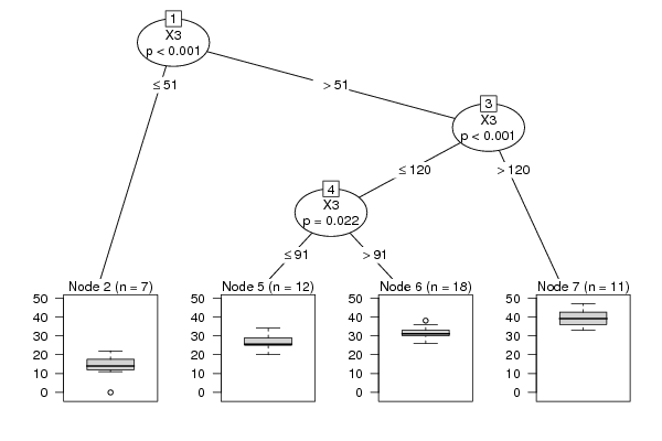
bitmap(file='test1.png')
plot(m)
dev.off()
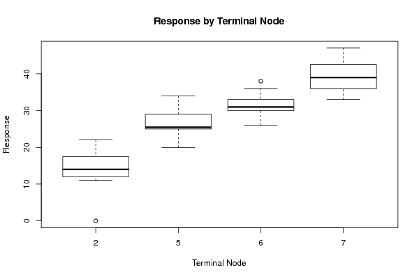
bitmap(file='test1a.png')
plot(x[,par1] ~ as.factor(where(m)),main='Response by Terminal Node',xlab='Terminal Node',ylab='Response')
dev.off()
if (par2 == 'none') {
forec <- predict(m)
result <- as.data.frame(cbind(x[,par1],forec,x[,par1]-forec))
colnames(result) <- c('Actuals','Forecasts','Residuals')
print(result)
}
if (par2 != 'none') {
print(cbind(as.factor(x[,par1]),predict(m)))
myt <- table(as.factor(x[,par1]),predict(m))
print(myt)
}
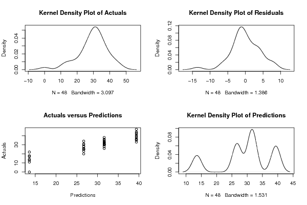
bitmap(file='test2.png')
if(par2=='none') {
op <- par(mfrow=c(2,2))
plot(density(result$Actuals),main='Kernel Density Plot of Actuals')
plot(density(result$Residuals),main='Kernel Density Plot of Residuals')
plot(result$Forecasts,result$Actuals,main='Actuals versus Predictions',xlab='Predictions',ylab='Actuals')
plot(density(result$Forecasts),main='Kernel Density Plot of Predictions')
par(op)
}
if(par2!='none') {
plot(myt,main='Confusion Matrix',xlab='Actual',ylab='Predicted')
}
dev.off()
if (par2 == 'none') {
detcoef <- cor(result$Forecasts,result$Actuals)
a<-table.start()
a<-table.row.start(a)
a<-table.element(a,'Goodness of Fit',2,TRUE)
a<-table.row.end(a)
a<-table.row.start(a)
a<-table.element(a,'Correlation',1,TRUE)
a<-table.element(a,round(detcoef,4))
a<-table.row.end(a)
a<-table.row.start(a)
a<-table.element(a,'R-squared',1,TRUE)
a<-table.element(a,round(detcoef*detcoef,4))
a<-table.row.end(a)
a<-table.row.start(a)
a<-table.element(a,'RMSE',1,TRUE)
a<-table.element(a,round(sqrt(mean((result$Residuals)^2)),4))
a<-table.row.end(a)
a<-table.end(a)
table.save(a,file='mytable1.tab')
a<-table.start()
a<-table.row.start(a)
a<-table.element(a,'Actuals, Predictions, and Residuals',4,TRUE)
a<-table.row.end(a)
a<-table.row.start(a)
a<-table.element(a,'#',header=TRUE)
a<-table.element(a,'Actuals',header=TRUE)
a<-table.element(a,'Forecasts',header=TRUE)
a<-table.element(a,'Residuals',header=TRUE)
a<-table.row.end(a)
for (i in 1:length(result$Actuals)) {
a<-table.row.start(a)
a<-table.element(a,i,header=TRUE)
a<-table.element(a,result$Actuals[i])
a<-table.element(a,result$Forecasts[i])
a<-table.element(a,result$Residuals[i])
a<-table.row.end(a)
}
a<-table.end(a)
table.save(a,file='mytable.tab')
}
if (par2 != 'none') {
a<-table.start()
a<-table.row.start(a)
a<-table.element(a,'Confusion Matrix (predicted in columns / actuals in rows)',par3+1,TRUE)
a<-table.row.end(a)
a<-table.row.start(a)
a<-table.element(a,'',1,TRUE)
for (i in 1:par3) {
a<-table.element(a,paste('C',i,sep=''),1,TRUE)
}
a<-table.row.end(a)
for (i in 1:par3) {
a<-table.row.start(a)
a<-table.element(a,paste('C',i,sep=''),1,TRUE)
for (j in 1:par3) {
a<-table.element(a,myt[i,j])
}
a<-table.row.end(a)
}
a<-table.end(a)
table.save(a,file='mytable2.tab')
}