Repository of Reproducible Computations

Free Statistics

of Irreproducible Research!

Author's title

Author

*The author of this computation has been verified*

R Software Module

rwasp_autocorrelation.wasp

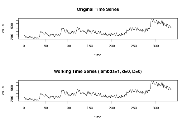
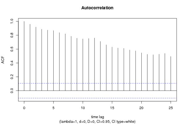
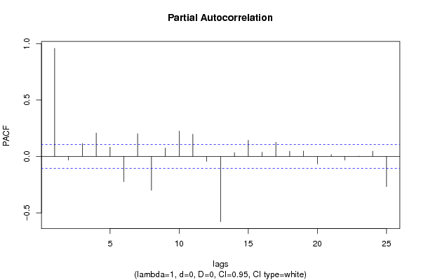
Title produced by software

(Partial) Autocorrelation Function

Date of computation

Fri, 23 Dec 2011 03:01:40 -0500

Cite this page as follows

Statistical Computations at FreeStatistics.org, Office for Research Development and Education, URL https://freestatistics.org/blog/index.php?v=date/2011/Dec/23/t1324627318lm0dcc3amenluiu.htm/, Retrieved Mon, 29 Apr 2024 18:32:26 +0000

Statistical Computations at FreeStatistics.org, Office for Research Development and Education, URL https://freestatistics.org/blog/index.php?pk=160176, Retrieved Mon, 29 Apr 2024 18:32:26 +0000

QR Codes:

Paste this QR Code to cite your computation.

Original text written by user:

IsPrivate?

No (this computation is public)

User-defined keywords

Estimated Impact

114

Family? (F = Feedback message, R = changed R code, M = changed R Module, P = changed Parameters, D = changed Data)

-     [Univariate Explorative Data Analysis] [Run Sequence gebo...] [2008-12-12 13:32:37] [76963dc1903f0f612b6153510a3818cf]
- R  D  [Univariate Explorative Data Analysis] [Run Sequence gebo...] [2008-12-17 12:14:40] [76963dc1903f0f612b6153510a3818cf]
-         [Univariate Explorative Data Analysis] [Run Sequence Plot...] [2008-12-22 18:19:51] [1ce0d16c8f4225c977b42c8fa93bc163]
- RMP       [Univariate Data Series] [Identifying Integ...] [2009-11-22 12:08:06] [b98453cac15ba1066b407e146608df68]
- RMPD        [(Partial) Autocorrelation Function] [] [2011-11-25 15:10:22] [b1eb71d4db1ceb5d347df987feb4a25e]
- R  D            [(Partial) Autocorrelation Function] [Paper] [2011-12-23 08:01:40] [8829043a11b4adcf2fcb2d15cd36bb4f] [Current]

Feedback Forum

Post a new message

Dataseries X:

Download CSV

Histogram

Boxplots

Summary of computational transaction
Raw Input	view raw input (R code)
Raw Output	view raw output of R engine
Computing time	1 seconds
R Server	'Gwilym Jenkins' @ jenkins.wessa.net

\begin{tabular}{lllllllll}
\hline
Summary of computational transaction \tabularnewline
Raw Input & view raw input (R code)  \tabularnewline
Raw Output & view raw output of R engine  \tabularnewline
Computing time & 1 seconds \tabularnewline
R Server & 'Gwilym Jenkins' @ jenkins.wessa.net \tabularnewline
\hline
\end{tabular}
%Source: https://freestatistics.org/blog/index.php?pk=160176&T=0

[TABLE]
[ROW][C]Summary of computational transaction[/C][/ROW]
[ROW][C]Raw Input[/C][C]view raw input (R code) [/C][/ROW]
[ROW][C]Raw Output[/C][C]view raw output of R engine [/C][/ROW]
[ROW][C]Computing time[/C][C]1 seconds[/C][/ROW]
[ROW][C]R Server[/C][C]'Gwilym Jenkins' @ jenkins.wessa.net[/C][/ROW]
[/TABLE]
Source: https://freestatistics.org/blog/index.php?pk=160176&T=0

Globally Unique Identifier (entire table): ba.freestatistics.org/blog/index.php?pk=160176&T=0

As an alternative you can also use a QR Code:

The GUIDs for individual cells are displayed in the table below:

Summary of computational transaction
Raw Input	view raw input (R code)
Raw Output	view raw output of R engine
Computing time	1 seconds
R Server	'Gwilym Jenkins' @ jenkins.wessa.net

Autocorrelation Function
Time lag k	ACF(k)	T-STAT	P-value
1	0.95934	17.585	0
2	0.917713	16.822	0
3	0.886931	16.2577	0
4	0.874058	16.0218	0
5	0.866642	15.8858	0
6	0.838102	15.3627	0
7	0.820179	15.0341	0
8	0.784503	14.3802	0
9	0.756819	13.8727	0
10	0.747443	13.7009	0
11	0.753162	13.8057	0
12	0.760259	13.9358	0
13	0.711061	13.034	0
14	0.66274	12.1482	0
15	0.629408	11.5372	0
16	0.615791	11.2876	0
17	0.610916	11.1983	0
18	0.588063	10.7794	0
19	0.575419	10.5476	0
20	0.546351	10.0148	0
21	0.525098	9.6252	0
22	0.519272	9.5184	0
23	0.526877	9.6578	0
24	0.537251	9.848	0
25	0.49414	9.0577	0

\begin{tabular}{lllllllll}
\hline
Autocorrelation Function \tabularnewline
Time lag k & ACF(k) & T-STAT & P-value \tabularnewline
1 & 0.95934 & 17.585 & 0 \tabularnewline
2 & 0.917713 & 16.822 & 0 \tabularnewline
3 & 0.886931 & 16.2577 & 0 \tabularnewline
4 & 0.874058 & 16.0218 & 0 \tabularnewline
5 & 0.866642 & 15.8858 & 0 \tabularnewline
6 & 0.838102 & 15.3627 & 0 \tabularnewline
7 & 0.820179 & 15.0341 & 0 \tabularnewline
8 & 0.784503 & 14.3802 & 0 \tabularnewline
9 & 0.756819 & 13.8727 & 0 \tabularnewline
10 & 0.747443 & 13.7009 & 0 \tabularnewline
11 & 0.753162 & 13.8057 & 0 \tabularnewline
12 & 0.760259 & 13.9358 & 0 \tabularnewline
13 & 0.711061 & 13.034 & 0 \tabularnewline
14 & 0.66274 & 12.1482 & 0 \tabularnewline
15 & 0.629408 & 11.5372 & 0 \tabularnewline
16 & 0.615791 & 11.2876 & 0 \tabularnewline
17 & 0.610916 & 11.1983 & 0 \tabularnewline
18 & 0.588063 & 10.7794 & 0 \tabularnewline
19 & 0.575419 & 10.5476 & 0 \tabularnewline
20 & 0.546351 & 10.0148 & 0 \tabularnewline
21 & 0.525098 & 9.6252 & 0 \tabularnewline
22 & 0.519272 & 9.5184 & 0 \tabularnewline
23 & 0.526877 & 9.6578 & 0 \tabularnewline
24 & 0.537251 & 9.848 & 0 \tabularnewline
25 & 0.49414 & 9.0577 & 0 \tabularnewline
\hline
\end{tabular}
%Source: https://freestatistics.org/blog/index.php?pk=160176&T=1

[TABLE]
[ROW][C]Autocorrelation Function[/C][/ROW]
[ROW][C]Time lag k[/C][C]ACF(k)[/C][C]T-STAT[/C][C]P-value[/C][/ROW]
[ROW][C]1[/C][C]0.95934[/C][C]17.585[/C][C]0[/C][/ROW]
[ROW][C]2[/C][C]0.917713[/C][C]16.822[/C][C]0[/C][/ROW]
[ROW][C]3[/C][C]0.886931[/C][C]16.2577[/C][C]0[/C][/ROW]
[ROW][C]4[/C][C]0.874058[/C][C]16.0218[/C][C]0[/C][/ROW]
[ROW][C]5[/C][C]0.866642[/C][C]15.8858[/C][C]0[/C][/ROW]
[ROW][C]6[/C][C]0.838102[/C][C]15.3627[/C][C]0[/C][/ROW]
[ROW][C]7[/C][C]0.820179[/C][C]15.0341[/C][C]0[/C][/ROW]
[ROW][C]8[/C][C]0.784503[/C][C]14.3802[/C][C]0[/C][/ROW]
[ROW][C]9[/C][C]0.756819[/C][C]13.8727[/C][C]0[/C][/ROW]
[ROW][C]10[/C][C]0.747443[/C][C]13.7009[/C][C]0[/C][/ROW]
[ROW][C]11[/C][C]0.753162[/C][C]13.8057[/C][C]0[/C][/ROW]
[ROW][C]12[/C][C]0.760259[/C][C]13.9358[/C][C]0[/C][/ROW]
[ROW][C]13[/C][C]0.711061[/C][C]13.034[/C][C]0[/C][/ROW]
[ROW][C]14[/C][C]0.66274[/C][C]12.1482[/C][C]0[/C][/ROW]
[ROW][C]15[/C][C]0.629408[/C][C]11.5372[/C][C]0[/C][/ROW]
[ROW][C]16[/C][C]0.615791[/C][C]11.2876[/C][C]0[/C][/ROW]
[ROW][C]17[/C][C]0.610916[/C][C]11.1983[/C][C]0[/C][/ROW]
[ROW][C]18[/C][C]0.588063[/C][C]10.7794[/C][C]0[/C][/ROW]
[ROW][C]19[/C][C]0.575419[/C][C]10.5476[/C][C]0[/C][/ROW]
[ROW][C]20[/C][C]0.546351[/C][C]10.0148[/C][C]0[/C][/ROW]
[ROW][C]21[/C][C]0.525098[/C][C]9.6252[/C][C]0[/C][/ROW]
[ROW][C]22[/C][C]0.519272[/C][C]9.5184[/C][C]0[/C][/ROW]
[ROW][C]23[/C][C]0.526877[/C][C]9.6578[/C][C]0[/C][/ROW]
[ROW][C]24[/C][C]0.537251[/C][C]9.848[/C][C]0[/C][/ROW]
[ROW][C]25[/C][C]0.49414[/C][C]9.0577[/C][C]0[/C][/ROW]
[/TABLE]
Source: https://freestatistics.org/blog/index.php?pk=160176&T=1

Globally Unique Identifier (entire table): ba.freestatistics.org/blog/index.php?pk=160176&T=1

As an alternative you can also use a QR Code:

The GUIDs for individual cells are displayed in the table below:

Autocorrelation Function
Time lag k	ACF(k)	T-STAT	P-value
1	0.95934	17.585	0
2	0.917713	16.822	0
3	0.886931	16.2577	0
4	0.874058	16.0218	0
5	0.866642	15.8858	0
6	0.838102	15.3627	0
7	0.820179	15.0341	0
8	0.784503	14.3802	0
9	0.756819	13.8727	0
10	0.747443	13.7009	0
11	0.753162	13.8057	0
12	0.760259	13.9358	0
13	0.711061	13.034	0
14	0.66274	12.1482	0
15	0.629408	11.5372	0
16	0.615791	11.2876	0
17	0.610916	11.1983	0
18	0.588063	10.7794	0
19	0.575419	10.5476	0
20	0.546351	10.0148	0
21	0.525098	9.6252	0
22	0.519272	9.5184	0
23	0.526877	9.6578	0
24	0.537251	9.848	0
25	0.49414	9.0577	0

Partial Autocorrelation Function
Time lag k	PACF(k)	T-STAT	P-value
1	0.95934	17.585	0
2	-0.032897	-0.603	0.273452
3	0.11472	2.1029	0.018111
4	0.207655	3.8064	8.4e-05
5	0.081533	1.4945	0.06799
6	-0.224186	-4.1094	2.5e-05
7	0.201995	3.7026	0.000125
8	-0.300406	-5.5065	0
9	0.07487	1.3724	0.085429
10	0.224988	4.1241	2.3e-05
11	0.196705	3.6057	0.000179
12	-0.043576	-0.7988	0.212494
13	-0.578538	-10.6048	0
14	0.034507	0.6325	0.26374
15	0.143892	2.6376	0.004369
16	0.037542	0.6882	0.245915
17	0.125292	2.2966	0.011127
18	0.046015	0.8435	0.199781
19	0.048184	0.8832	0.188873
20	-0.067122	-1.2304	0.10971
21	0.016201	0.297	0.383339
22	-0.032792	-0.6011	0.274096
23	0.000875	0.016	0.493606
24	0.046247	0.8477	0.198599
25	-0.267504	-4.9034	1e-06

\begin{tabular}{lllllllll}
\hline
Partial Autocorrelation Function \tabularnewline
Time lag k & PACF(k) & T-STAT & P-value \tabularnewline
1 & 0.95934 & 17.585 & 0 \tabularnewline
2 & -0.032897 & -0.603 & 0.273452 \tabularnewline
3 & 0.11472 & 2.1029 & 0.018111 \tabularnewline
4 & 0.207655 & 3.8064 & 8.4e-05 \tabularnewline
5 & 0.081533 & 1.4945 & 0.06799 \tabularnewline
6 & -0.224186 & -4.1094 & 2.5e-05 \tabularnewline
7 & 0.201995 & 3.7026 & 0.000125 \tabularnewline
8 & -0.300406 & -5.5065 & 0 \tabularnewline
9 & 0.07487 & 1.3724 & 0.085429 \tabularnewline
10 & 0.224988 & 4.1241 & 2.3e-05 \tabularnewline
11 & 0.196705 & 3.6057 & 0.000179 \tabularnewline
12 & -0.043576 & -0.7988 & 0.212494 \tabularnewline
13 & -0.578538 & -10.6048 & 0 \tabularnewline
14 & 0.034507 & 0.6325 & 0.26374 \tabularnewline
15 & 0.143892 & 2.6376 & 0.004369 \tabularnewline
16 & 0.037542 & 0.6882 & 0.245915 \tabularnewline
17 & 0.125292 & 2.2966 & 0.011127 \tabularnewline
18 & 0.046015 & 0.8435 & 0.199781 \tabularnewline
19 & 0.048184 & 0.8832 & 0.188873 \tabularnewline
20 & -0.067122 & -1.2304 & 0.10971 \tabularnewline
21 & 0.016201 & 0.297 & 0.383339 \tabularnewline
22 & -0.032792 & -0.6011 & 0.274096 \tabularnewline
23 & 0.000875 & 0.016 & 0.493606 \tabularnewline
24 & 0.046247 & 0.8477 & 0.198599 \tabularnewline
25 & -0.267504 & -4.9034 & 1e-06 \tabularnewline
\hline
\end{tabular}
%Source: https://freestatistics.org/blog/index.php?pk=160176&T=2

[TABLE]
[ROW][C]Partial Autocorrelation Function[/C][/ROW]
[ROW][C]Time lag k[/C][C]PACF(k)[/C][C]T-STAT[/C][C]P-value[/C][/ROW]
[ROW][C]1[/C][C]0.95934[/C][C]17.585[/C][C]0[/C][/ROW]
[ROW][C]2[/C][C]-0.032897[/C][C]-0.603[/C][C]0.273452[/C][/ROW]
[ROW][C]3[/C][C]0.11472[/C][C]2.1029[/C][C]0.018111[/C][/ROW]
[ROW][C]4[/C][C]0.207655[/C][C]3.8064[/C][C]8.4e-05[/C][/ROW]
[ROW][C]5[/C][C]0.081533[/C][C]1.4945[/C][C]0.06799[/C][/ROW]
[ROW][C]6[/C][C]-0.224186[/C][C]-4.1094[/C][C]2.5e-05[/C][/ROW]
[ROW][C]7[/C][C]0.201995[/C][C]3.7026[/C][C]0.000125[/C][/ROW]
[ROW][C]8[/C][C]-0.300406[/C][C]-5.5065[/C][C]0[/C][/ROW]
[ROW][C]9[/C][C]0.07487[/C][C]1.3724[/C][C]0.085429[/C][/ROW]
[ROW][C]10[/C][C]0.224988[/C][C]4.1241[/C][C]2.3e-05[/C][/ROW]
[ROW][C]11[/C][C]0.196705[/C][C]3.6057[/C][C]0.000179[/C][/ROW]
[ROW][C]12[/C][C]-0.043576[/C][C]-0.7988[/C][C]0.212494[/C][/ROW]
[ROW][C]13[/C][C]-0.578538[/C][C]-10.6048[/C][C]0[/C][/ROW]
[ROW][C]14[/C][C]0.034507[/C][C]0.6325[/C][C]0.26374[/C][/ROW]
[ROW][C]15[/C][C]0.143892[/C][C]2.6376[/C][C]0.004369[/C][/ROW]
[ROW][C]16[/C][C]0.037542[/C][C]0.6882[/C][C]0.245915[/C][/ROW]
[ROW][C]17[/C][C]0.125292[/C][C]2.2966[/C][C]0.011127[/C][/ROW]
[ROW][C]18[/C][C]0.046015[/C][C]0.8435[/C][C]0.199781[/C][/ROW]
[ROW][C]19[/C][C]0.048184[/C][C]0.8832[/C][C]0.188873[/C][/ROW]
[ROW][C]20[/C][C]-0.067122[/C][C]-1.2304[/C][C]0.10971[/C][/ROW]
[ROW][C]21[/C][C]0.016201[/C][C]0.297[/C][C]0.383339[/C][/ROW]
[ROW][C]22[/C][C]-0.032792[/C][C]-0.6011[/C][C]0.274096[/C][/ROW]
[ROW][C]23[/C][C]0.000875[/C][C]0.016[/C][C]0.493606[/C][/ROW]
[ROW][C]24[/C][C]0.046247[/C][C]0.8477[/C][C]0.198599[/C][/ROW]
[ROW][C]25[/C][C]-0.267504[/C][C]-4.9034[/C][C]1e-06[/C][/ROW]
[/TABLE]
Source: https://freestatistics.org/blog/index.php?pk=160176&T=2

Globally Unique Identifier (entire table): ba.freestatistics.org/blog/index.php?pk=160176&T=2

As an alternative you can also use a QR Code:

The GUIDs for individual cells are displayed in the table below:

Partial Autocorrelation Function
Time lag k	PACF(k)	T-STAT	P-value
1	0.95934	17.585	0
2	-0.032897	-0.603	0.273452
3	0.11472	2.1029	0.018111
4	0.207655	3.8064	8.4e-05
5	0.081533	1.4945	0.06799
6	-0.224186	-4.1094	2.5e-05
7	0.201995	3.7026	0.000125
8	-0.300406	-5.5065	0
9	0.07487	1.3724	0.085429
10	0.224988	4.1241	2.3e-05
11	0.196705	3.6057	0.000179
12	-0.043576	-0.7988	0.212494
13	-0.578538	-10.6048	0
14	0.034507	0.6325	0.26374
15	0.143892	2.6376	0.004369
16	0.037542	0.6882	0.245915
17	0.125292	2.2966	0.011127
18	0.046015	0.8435	0.199781
19	0.048184	0.8832	0.188873
20	-0.067122	-1.2304	0.10971
21	0.016201	0.297	0.383339
22	-0.032792	-0.6011	0.274096
23	0.000875	0.016	0.493606
24	0.046247	0.8477	0.198599
25	-0.267504	-4.9034	1e-06

Figure 1

PNG link

Postscript link

PDF link

Figure 2

PNG link

Postscript link

PDF link

Figure 3

PNG link

Postscript link

PDF link

Parameters (Session):

par1 = Default ; par2 = 1 ; par3 = 0 ; par4 = 0 ; par5 = 12 ; par6 = White Noise ; par7 = 0.95 ;

Parameters (R input):

par1 = Default ; par2 = 1 ; par3 = 0 ; par4 = 0 ; par5 = 12 ; par6 = White Noise ; par7 = 0.95 ; par8 = ;

R code (references can be found in the software module):

if (par1 == 'Default') {
par1 = 10*log10(length(x))
} else {
par1 <- as.numeric(par1)
}
par2 <- as.numeric(par2)
par3 <- as.numeric(par3)
par4 <- as.numeric(par4)
par5 <- as.numeric(par5)
if (par6 == 'White Noise') par6 <- 'white' else par6 <- 'ma'
par7 <- as.numeric(par7)
if (par8 != '') par8 <- as.numeric(par8)
ox <- x
if (par8 == '') {
if (par2 == 0) {
x <- log(x)
} else {
x <- (x ^ par2 - 1) / par2
}
} else {
x <- log(x,base=par8)
}
if (par3 > 0) x <- diff(x,lag=1,difference=par3)
if (par4 > 0) x <- diff(x,lag=par5,difference=par4)
bitmap(file='picts.png')
op <- par(mfrow=c(2,1))
plot(ox,type='l',main='Original Time Series',xlab='time',ylab='value')
if (par8=='') {
mytitle <- paste('Working Time Series (lambda=',par2,', d=',par3,', D=',par4,')',sep='')
mysub <- paste('(lambda=',par2,', d=',par3,', D=',par4,', CI=', par7, ', CI type=',par6,')',sep='')
} else {
mytitle <- paste('Working Time Series (base=',par8,', d=',par3,', D=',par4,')',sep='')
mysub <- paste('(base=',par8,', d=',par3,', D=',par4,', CI=', par7, ', CI type=',par6,')',sep='')
}
plot(x,type='l', main=mytitle,xlab='time',ylab='value')
par(op)
dev.off()
bitmap(file='pic1.png')
racf <- acf(x, par1, main='Autocorrelation', xlab='time lag', ylab='ACF', ci.type=par6, ci=par7, sub=mysub)
dev.off()
bitmap(file='pic2.png')
rpacf <- pacf(x,par1,main='Partial Autocorrelation',xlab='lags',ylab='PACF',sub=mysub)
dev.off()
(myacf <- c(racf$acf))
(mypacf <- c(rpacf$acf))
lengthx <- length(x)
sqrtn <- sqrt(lengthx)
load(file='createtable')
a<-table.start()
a<-table.row.start(a)
a<-table.element(a,'Autocorrelation Function',4,TRUE)
a<-table.row.end(a)
a<-table.row.start(a)
a<-table.element(a,'Time lag k',header=TRUE)
a<-table.element(a,hyperlink('basics.htm','ACF(k)','click here for more information about the Autocorrelation Function'),header=TRUE)
a<-table.element(a,'T-STAT',header=TRUE)
a<-table.element(a,'P-value',header=TRUE)
a<-table.row.end(a)
for (i in 2:(par1+1)) {
a<-table.row.start(a)
a<-table.element(a,i-1,header=TRUE)
a<-table.element(a,round(myacf[i],6))
mytstat <- myacf[i]*sqrtn
a<-table.element(a,round(mytstat,4))
a<-table.element(a,round(1-pt(abs(mytstat),lengthx),6))
a<-table.row.end(a)
}
a<-table.end(a)
table.save(a,file='mytable.tab')
a<-table.start()
a<-table.row.start(a)
a<-table.element(a,'Partial Autocorrelation Function',4,TRUE)
a<-table.row.end(a)
a<-table.row.start(a)
a<-table.element(a,'Time lag k',header=TRUE)
a<-table.element(a,hyperlink('basics.htm','PACF(k)','click here for more information about the Partial Autocorrelation Function'),header=TRUE)
a<-table.element(a,'T-STAT',header=TRUE)
a<-table.element(a,'P-value',header=TRUE)
a<-table.row.end(a)
for (i in 1:par1) {
a<-table.row.start(a)
a<-table.element(a,i,header=TRUE)
a<-table.element(a,round(mypacf[i],6))
mytstat <- mypacf[i]*sqrtn
a<-table.element(a,round(mytstat,4))
a<-table.element(a,round(1-pt(abs(mytstat),lengthx),6))
a<-table.row.end(a)
}
a<-table.end(a)
table.save(a,file='mytable1.tab')

Free Statistics

Description of Statistical Computation

Tree of Dependent Computations

Dataset

Tables (Output of Computation)

Figures (Output of Computation)

Input Parameters & R Code