Repository of Reproducible Computations

Free Statistics

of Irreproducible Research!

Author's title

Author

*The author of this computation has been verified*

R Software Module

rwasp_autocorrelation.wasp

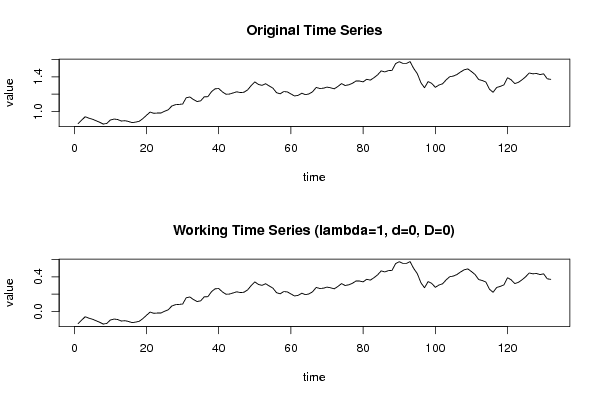
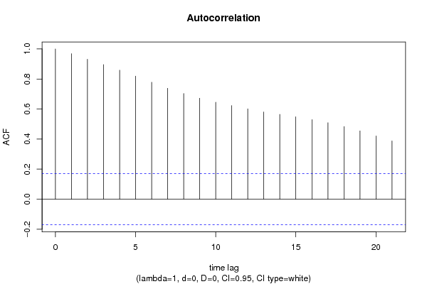
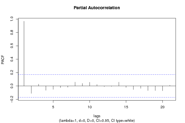
Title produced by software

(Partial) Autocorrelation Function

Date of computation

Wed, 21 Dec 2011 06:30:33 -0500

Cite this page as follows

Statistical Computations at FreeStatistics.org, Office for Research Development and Education, URL https://freestatistics.org/blog/index.php?v=date/2011/Dec/21/t1324467054ym3fytx6pgf9iqu.htm/, Retrieved Tue, 07 May 2024 05:13:32 +0000

Statistical Computations at FreeStatistics.org, Office for Research Development and Education, URL https://freestatistics.org/blog/index.php?pk=158518, Retrieved Tue, 07 May 2024 05:13:32 +0000

QR Codes:

Paste this QR Code to cite your computation.

Original text written by user:

IsPrivate?

No (this computation is public)

User-defined keywords

Estimated Impact

129

Family? (F = Feedback message, R = changed R code, M = changed R Module, P = changed Parameters, D = changed Data)

-     [Univariate Data Series] [web traffic] [2010-10-19 15:13:07] [b98453cac15ba1066b407e146608df68]
- RMP   [Variance Reduction Matrix] [Traffic] [2010-11-29 09:57:15] [b98453cac15ba1066b407e146608df68]
- RM      [Standard Deviation-Mean Plot] [Traffic] [2010-11-29 11:05:08] [b98453cac15ba1066b407e146608df68]
- RMP       [ARIMA Forecasting] [Traffic] [2010-11-29 21:10:32] [b98453cac15ba1066b407e146608df68]
- R PD        [ARIMA Forecasting] [] [2011-12-06 10:39:07] [aba4febe8a2e49e81bdc61a6c01f5c21]
-   PD          [ARIMA Forecasting] [] [2011-12-20 15:47:34] [aba4febe8a2e49e81bdc61a6c01f5c21]
- R               [ARIMA Forecasting] [ARIMA Forecasting CV] [2011-12-20 15:48:10] [aba4febe8a2e49e81bdc61a6c01f5c21]
- RMPD              [ARIMA Backward Selection] [paper arima backw...] [2011-12-21 10:36:30] [aba4febe8a2e49e81bdc61a6c01f5c21]
- RM D                  [(Partial) Autocorrelation Function] [Paper ACF wisselk...] [2011-12-21 11:30:33] [3627de22d386f4cb93d383ef7c1ade7f] [Current]

Feedback Forum

Post a new message

Dataseries X:

Download CSV

Histogram

Boxplots

Summary of computational transaction
Raw Input	view raw input (R code)
Raw Output	view raw output of R engine
Computing time	2 seconds
R Server	'AstonUniversity' @ aston.wessa.net

\begin{tabular}{lllllllll}
\hline
Summary of computational transaction \tabularnewline
Raw Input & view raw input (R code)  \tabularnewline
Raw Output & view raw output of R engine  \tabularnewline
Computing time & 2 seconds \tabularnewline
R Server & 'AstonUniversity' @ aston.wessa.net \tabularnewline
\hline
\end{tabular}
%Source: https://freestatistics.org/blog/index.php?pk=158518&T=0

[TABLE]
[ROW][C]Summary of computational transaction[/C][/ROW]
[ROW][C]Raw Input[/C][C]view raw input (R code) [/C][/ROW]
[ROW][C]Raw Output[/C][C]view raw output of R engine [/C][/ROW]
[ROW][C]Computing time[/C][C]2 seconds[/C][/ROW]
[ROW][C]R Server[/C][C]'AstonUniversity' @ aston.wessa.net[/C][/ROW]
[/TABLE]
Source: https://freestatistics.org/blog/index.php?pk=158518&T=0

Globally Unique Identifier (entire table): ba.freestatistics.org/blog/index.php?pk=158518&T=0

As an alternative you can also use a QR Code:

The GUIDs for individual cells are displayed in the table below:

Summary of computational transaction
Raw Input	view raw input (R code)
Raw Output	view raw output of R engine
Computing time	2 seconds
R Server	'AstonUniversity' @ aston.wessa.net

Autocorrelation Function
Time lag k	ACF(k)	T-STAT	P-value
1	0.968521	11.1275	0
2	0.931145	10.698	0
3	0.89609	10.2953	0
4	0.858655	9.8652	0
5	0.818717	9.4063	0
6	0.778368	8.9428	0
7	0.738269	8.4821	0
8	0.702961	8.0764	0
9	0.672022	7.7209	0
10	0.645871	7.4205	0
11	0.622908	7.1567	0
12	0.601041	6.9054	0
13	0.580256	6.6666	0
14	0.56452	6.4858	0
15	0.548951	6.307	0
16	0.530044	6.0897	0
17	0.5089	5.8468	0
18	0.483962	5.5603	0
19	0.454619	5.2232	0
20	0.421066	4.8377	2e-06
21	0.387912	4.4568	9e-06

\begin{tabular}{lllllllll}
\hline
Autocorrelation Function \tabularnewline
Time lag k & ACF(k) & T-STAT & P-value \tabularnewline
1 & 0.968521 & 11.1275 & 0 \tabularnewline
2 & 0.931145 & 10.698 & 0 \tabularnewline
3 & 0.89609 & 10.2953 & 0 \tabularnewline
4 & 0.858655 & 9.8652 & 0 \tabularnewline
5 & 0.818717 & 9.4063 & 0 \tabularnewline
6 & 0.778368 & 8.9428 & 0 \tabularnewline
7 & 0.738269 & 8.4821 & 0 \tabularnewline
8 & 0.702961 & 8.0764 & 0 \tabularnewline
9 & 0.672022 & 7.7209 & 0 \tabularnewline
10 & 0.645871 & 7.4205 & 0 \tabularnewline
11 & 0.622908 & 7.1567 & 0 \tabularnewline
12 & 0.601041 & 6.9054 & 0 \tabularnewline
13 & 0.580256 & 6.6666 & 0 \tabularnewline
14 & 0.56452 & 6.4858 & 0 \tabularnewline
15 & 0.548951 & 6.307 & 0 \tabularnewline
16 & 0.530044 & 6.0897 & 0 \tabularnewline
17 & 0.5089 & 5.8468 & 0 \tabularnewline
18 & 0.483962 & 5.5603 & 0 \tabularnewline
19 & 0.454619 & 5.2232 & 0 \tabularnewline
20 & 0.421066 & 4.8377 & 2e-06 \tabularnewline
21 & 0.387912 & 4.4568 & 9e-06 \tabularnewline
\hline
\end{tabular}
%Source: https://freestatistics.org/blog/index.php?pk=158518&T=1

[TABLE]
[ROW][C]Autocorrelation Function[/C][/ROW]
[ROW][C]Time lag k[/C][C]ACF(k)[/C][C]T-STAT[/C][C]P-value[/C][/ROW]
[ROW][C]1[/C][C]0.968521[/C][C]11.1275[/C][C]0[/C][/ROW]
[ROW][C]2[/C][C]0.931145[/C][C]10.698[/C][C]0[/C][/ROW]
[ROW][C]3[/C][C]0.89609[/C][C]10.2953[/C][C]0[/C][/ROW]
[ROW][C]4[/C][C]0.858655[/C][C]9.8652[/C][C]0[/C][/ROW]
[ROW][C]5[/C][C]0.818717[/C][C]9.4063[/C][C]0[/C][/ROW]
[ROW][C]6[/C][C]0.778368[/C][C]8.9428[/C][C]0[/C][/ROW]
[ROW][C]7[/C][C]0.738269[/C][C]8.4821[/C][C]0[/C][/ROW]
[ROW][C]8[/C][C]0.702961[/C][C]8.0764[/C][C]0[/C][/ROW]
[ROW][C]9[/C][C]0.672022[/C][C]7.7209[/C][C]0[/C][/ROW]
[ROW][C]10[/C][C]0.645871[/C][C]7.4205[/C][C]0[/C][/ROW]
[ROW][C]11[/C][C]0.622908[/C][C]7.1567[/C][C]0[/C][/ROW]
[ROW][C]12[/C][C]0.601041[/C][C]6.9054[/C][C]0[/C][/ROW]
[ROW][C]13[/C][C]0.580256[/C][C]6.6666[/C][C]0[/C][/ROW]
[ROW][C]14[/C][C]0.56452[/C][C]6.4858[/C][C]0[/C][/ROW]
[ROW][C]15[/C][C]0.548951[/C][C]6.307[/C][C]0[/C][/ROW]
[ROW][C]16[/C][C]0.530044[/C][C]6.0897[/C][C]0[/C][/ROW]
[ROW][C]17[/C][C]0.5089[/C][C]5.8468[/C][C]0[/C][/ROW]
[ROW][C]18[/C][C]0.483962[/C][C]5.5603[/C][C]0[/C][/ROW]
[ROW][C]19[/C][C]0.454619[/C][C]5.2232[/C][C]0[/C][/ROW]
[ROW][C]20[/C][C]0.421066[/C][C]4.8377[/C][C]2e-06[/C][/ROW]
[ROW][C]21[/C][C]0.387912[/C][C]4.4568[/C][C]9e-06[/C][/ROW]
[/TABLE]
Source: https://freestatistics.org/blog/index.php?pk=158518&T=1

Globally Unique Identifier (entire table): ba.freestatistics.org/blog/index.php?pk=158518&T=1

As an alternative you can also use a QR Code:

The GUIDs for individual cells are displayed in the table below:

Autocorrelation Function
Time lag k	ACF(k)	T-STAT	P-value
1	0.968521	11.1275	0
2	0.931145	10.698	0
3	0.89609	10.2953	0
4	0.858655	9.8652	0
5	0.818717	9.4063	0
6	0.778368	8.9428	0
7	0.738269	8.4821	0
8	0.702961	8.0764	0
9	0.672022	7.7209	0
10	0.645871	7.4205	0
11	0.622908	7.1567	0
12	0.601041	6.9054	0
13	0.580256	6.6666	0
14	0.56452	6.4858	0
15	0.548951	6.307	0
16	0.530044	6.0897	0
17	0.5089	5.8468	0
18	0.483962	5.5603	0
19	0.454619	5.2232	0
20	0.421066	4.8377	2e-06
21	0.387912	4.4568	9e-06

Partial Autocorrelation Function
Time lag k	PACF(k)	T-STAT	P-value
1	0.968521	11.1275	0
2	-0.111159	-1.2771	0.101901
3	0.027281	0.3134	0.377224
4	-0.065351	-0.7508	0.227045
5	-0.05124	-0.5887	0.278534
6	-0.025552	-0.2936	0.384773
7	-0.01923	-0.2209	0.412744
8	0.057462	0.6602	0.255141
9	0.038261	0.4396	0.330477
10	0.055387	0.6363	0.262826
11	0.021844	0.251	0.401113
12	-0.009294	-0.1068	0.457562
13	-0.006835	-0.0785	0.468761
14	0.057331	0.6587	0.255624
15	-0.022279	-0.256	0.399187
16	-0.053642	-0.6163	0.26938
17	-0.036312	-0.4172	0.338606
18	-0.069228	-0.7954	0.213914
19	-0.06947	-0.7981	0.213109
20	-0.072053	-0.8278	0.204632
21	0.010603	0.1218	0.451612

\begin{tabular}{lllllllll}
\hline
Partial Autocorrelation Function \tabularnewline
Time lag k & PACF(k) & T-STAT & P-value \tabularnewline
1 & 0.968521 & 11.1275 & 0 \tabularnewline
2 & -0.111159 & -1.2771 & 0.101901 \tabularnewline
3 & 0.027281 & 0.3134 & 0.377224 \tabularnewline
4 & -0.065351 & -0.7508 & 0.227045 \tabularnewline
5 & -0.05124 & -0.5887 & 0.278534 \tabularnewline
6 & -0.025552 & -0.2936 & 0.384773 \tabularnewline
7 & -0.01923 & -0.2209 & 0.412744 \tabularnewline
8 & 0.057462 & 0.6602 & 0.255141 \tabularnewline
9 & 0.038261 & 0.4396 & 0.330477 \tabularnewline
10 & 0.055387 & 0.6363 & 0.262826 \tabularnewline
11 & 0.021844 & 0.251 & 0.401113 \tabularnewline
12 & -0.009294 & -0.1068 & 0.457562 \tabularnewline
13 & -0.006835 & -0.0785 & 0.468761 \tabularnewline
14 & 0.057331 & 0.6587 & 0.255624 \tabularnewline
15 & -0.022279 & -0.256 & 0.399187 \tabularnewline
16 & -0.053642 & -0.6163 & 0.26938 \tabularnewline
17 & -0.036312 & -0.4172 & 0.338606 \tabularnewline
18 & -0.069228 & -0.7954 & 0.213914 \tabularnewline
19 & -0.06947 & -0.7981 & 0.213109 \tabularnewline
20 & -0.072053 & -0.8278 & 0.204632 \tabularnewline
21 & 0.010603 & 0.1218 & 0.451612 \tabularnewline
\hline
\end{tabular}
%Source: https://freestatistics.org/blog/index.php?pk=158518&T=2

[TABLE]
[ROW][C]Partial Autocorrelation Function[/C][/ROW]
[ROW][C]Time lag k[/C][C]PACF(k)[/C][C]T-STAT[/C][C]P-value[/C][/ROW]
[ROW][C]1[/C][C]0.968521[/C][C]11.1275[/C][C]0[/C][/ROW]
[ROW][C]2[/C][C]-0.111159[/C][C]-1.2771[/C][C]0.101901[/C][/ROW]
[ROW][C]3[/C][C]0.027281[/C][C]0.3134[/C][C]0.377224[/C][/ROW]
[ROW][C]4[/C][C]-0.065351[/C][C]-0.7508[/C][C]0.227045[/C][/ROW]
[ROW][C]5[/C][C]-0.05124[/C][C]-0.5887[/C][C]0.278534[/C][/ROW]
[ROW][C]6[/C][C]-0.025552[/C][C]-0.2936[/C][C]0.384773[/C][/ROW]
[ROW][C]7[/C][C]-0.01923[/C][C]-0.2209[/C][C]0.412744[/C][/ROW]
[ROW][C]8[/C][C]0.057462[/C][C]0.6602[/C][C]0.255141[/C][/ROW]
[ROW][C]9[/C][C]0.038261[/C][C]0.4396[/C][C]0.330477[/C][/ROW]
[ROW][C]10[/C][C]0.055387[/C][C]0.6363[/C][C]0.262826[/C][/ROW]
[ROW][C]11[/C][C]0.021844[/C][C]0.251[/C][C]0.401113[/C][/ROW]
[ROW][C]12[/C][C]-0.009294[/C][C]-0.1068[/C][C]0.457562[/C][/ROW]
[ROW][C]13[/C][C]-0.006835[/C][C]-0.0785[/C][C]0.468761[/C][/ROW]
[ROW][C]14[/C][C]0.057331[/C][C]0.6587[/C][C]0.255624[/C][/ROW]
[ROW][C]15[/C][C]-0.022279[/C][C]-0.256[/C][C]0.399187[/C][/ROW]
[ROW][C]16[/C][C]-0.053642[/C][C]-0.6163[/C][C]0.26938[/C][/ROW]
[ROW][C]17[/C][C]-0.036312[/C][C]-0.4172[/C][C]0.338606[/C][/ROW]
[ROW][C]18[/C][C]-0.069228[/C][C]-0.7954[/C][C]0.213914[/C][/ROW]
[ROW][C]19[/C][C]-0.06947[/C][C]-0.7981[/C][C]0.213109[/C][/ROW]
[ROW][C]20[/C][C]-0.072053[/C][C]-0.8278[/C][C]0.204632[/C][/ROW]
[ROW][C]21[/C][C]0.010603[/C][C]0.1218[/C][C]0.451612[/C][/ROW]
[/TABLE]
Source: https://freestatistics.org/blog/index.php?pk=158518&T=2

Globally Unique Identifier (entire table): ba.freestatistics.org/blog/index.php?pk=158518&T=2

As an alternative you can also use a QR Code:

The GUIDs for individual cells are displayed in the table below:

Partial Autocorrelation Function
Time lag k	PACF(k)	T-STAT	P-value
1	0.968521	11.1275	0
2	-0.111159	-1.2771	0.101901
3	0.027281	0.3134	0.377224
4	-0.065351	-0.7508	0.227045
5	-0.05124	-0.5887	0.278534
6	-0.025552	-0.2936	0.384773
7	-0.01923	-0.2209	0.412744
8	0.057462	0.6602	0.255141
9	0.038261	0.4396	0.330477
10	0.055387	0.6363	0.262826
11	0.021844	0.251	0.401113
12	-0.009294	-0.1068	0.457562
13	-0.006835	-0.0785	0.468761
14	0.057331	0.6587	0.255624
15	-0.022279	-0.256	0.399187
16	-0.053642	-0.6163	0.26938
17	-0.036312	-0.4172	0.338606
18	-0.069228	-0.7954	0.213914
19	-0.06947	-0.7981	0.213109
20	-0.072053	-0.8278	0.204632
21	0.010603	0.1218	0.451612

Figure 1

PNG link

Postscript link

PDF link

Figure 2

PNG link

Postscript link

PDF link

Figure 3

PNG link

Postscript link

PDF link

Parameters (Session):

par1 = 12 ;

Parameters (R input):

par1 = Default ; par2 = 1 ; par3 = 0 ; par4 = 0 ; par5 = 12 ; par6 = White Noise ; par7 = 0.95 ; par8 = ;

R code (references can be found in the software module):

if (par1 == 'Default') {
par1 = 10*log10(length(x))
} else {
par1 <- as.numeric(par1)
}
par2 <- as.numeric(par2)
par3 <- as.numeric(par3)
par4 <- as.numeric(par4)
par5 <- as.numeric(par5)
if (par6 == 'White Noise') par6 <- 'white' else par6 <- 'ma'
par7 <- as.numeric(par7)
if (par8 != '') par8 <- as.numeric(par8)
ox <- x
if (par8 == '') {
if (par2 == 0) {
x <- log(x)
} else {
x <- (x ^ par2 - 1) / par2
}
} else {
x <- log(x,base=par8)
}
if (par3 > 0) x <- diff(x,lag=1,difference=par3)
if (par4 > 0) x <- diff(x,lag=par5,difference=par4)
bitmap(file='picts.png')
op <- par(mfrow=c(2,1))
plot(ox,type='l',main='Original Time Series',xlab='time',ylab='value')
if (par8=='') {
mytitle <- paste('Working Time Series (lambda=',par2,', d=',par3,', D=',par4,')',sep='')
mysub <- paste('(lambda=',par2,', d=',par3,', D=',par4,', CI=', par7, ', CI type=',par6,')',sep='')
} else {
mytitle <- paste('Working Time Series (base=',par8,', d=',par3,', D=',par4,')',sep='')
mysub <- paste('(base=',par8,', d=',par3,', D=',par4,', CI=', par7, ', CI type=',par6,')',sep='')
}
plot(x,type='l', main=mytitle,xlab='time',ylab='value')
par(op)
dev.off()
bitmap(file='pic1.png')
racf <- acf(x, par1, main='Autocorrelation', xlab='time lag', ylab='ACF', ci.type=par6, ci=par7, sub=mysub)
dev.off()
bitmap(file='pic2.png')
rpacf <- pacf(x,par1,main='Partial Autocorrelation',xlab='lags',ylab='PACF',sub=mysub)
dev.off()
(myacf <- c(racf$acf))
(mypacf <- c(rpacf$acf))
lengthx <- length(x)
sqrtn <- sqrt(lengthx)
load(file='createtable')
a<-table.start()
a<-table.row.start(a)
a<-table.element(a,'Autocorrelation Function',4,TRUE)
a<-table.row.end(a)
a<-table.row.start(a)
a<-table.element(a,'Time lag k',header=TRUE)
a<-table.element(a,hyperlink('basics.htm','ACF(k)','click here for more information about the Autocorrelation Function'),header=TRUE)
a<-table.element(a,'T-STAT',header=TRUE)
a<-table.element(a,'P-value',header=TRUE)
a<-table.row.end(a)
for (i in 2:(par1+1)) {
a<-table.row.start(a)
a<-table.element(a,i-1,header=TRUE)
a<-table.element(a,round(myacf[i],6))
mytstat <- myacf[i]*sqrtn
a<-table.element(a,round(mytstat,4))
a<-table.element(a,round(1-pt(abs(mytstat),lengthx),6))
a<-table.row.end(a)
}
a<-table.end(a)
table.save(a,file='mytable.tab')
a<-table.start()
a<-table.row.start(a)
a<-table.element(a,'Partial Autocorrelation Function',4,TRUE)
a<-table.row.end(a)
a<-table.row.start(a)
a<-table.element(a,'Time lag k',header=TRUE)
a<-table.element(a,hyperlink('basics.htm','PACF(k)','click here for more information about the Partial Autocorrelation Function'),header=TRUE)
a<-table.element(a,'T-STAT',header=TRUE)
a<-table.element(a,'P-value',header=TRUE)
a<-table.row.end(a)
for (i in 1:par1) {
a<-table.row.start(a)
a<-table.element(a,i,header=TRUE)
a<-table.element(a,round(mypacf[i],6))
mytstat <- mypacf[i]*sqrtn
a<-table.element(a,round(mytstat,4))
a<-table.element(a,round(1-pt(abs(mytstat),lengthx),6))
a<-table.row.end(a)
}
a<-table.end(a)
table.save(a,file='mytable1.tab')

Free Statistics

Description of Statistical Computation

Tree of Dependent Computations

Dataset

Tables (Output of Computation)

Figures (Output of Computation)

Input Parameters & R Code