Repository of Reproducible Computations

Free Statistics

of Irreproducible Research!

Author's title

Author

*The author of this computation has been verified*

R Software Module

rwasp_autocorrelation.wasp

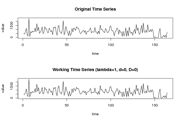
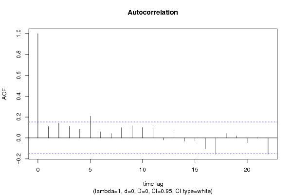
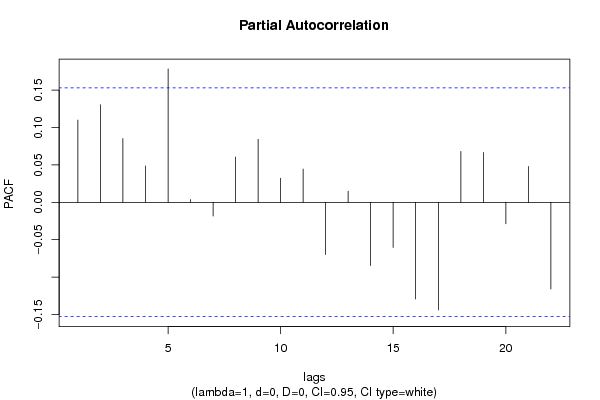
Title produced by software

(Partial) Autocorrelation Function

Date of computation

Wed, 21 Dec 2011 04:45:21 -0500

Cite this page as follows

Statistical Computations at FreeStatistics.org, Office for Research Development and Education, URL https://freestatistics.org/blog/index.php?v=date/2011/Dec/21/t13244607375yphxlijvofaq3y.htm/, Retrieved Tue, 07 May 2024 17:15:42 +0000

Statistical Computations at FreeStatistics.org, Office for Research Development and Education, URL https://freestatistics.org/blog/index.php?pk=158393, Retrieved Tue, 07 May 2024 17:15:42 +0000

QR Codes:

Paste this QR Code to cite your computation.

Original text written by user:

IsPrivate?

No (this computation is public)

User-defined keywords

Estimated Impact

131

Family? (F = Feedback message, R = changed R code, M = changed R Module, P = changed Parameters, D = changed Data)

-     [Univariate Data Series] [web traffic] [2010-10-19 15:13:07] [b98453cac15ba1066b407e146608df68]
- RMP   [Variance Reduction Matrix] [Traffic] [2010-11-29 09:57:15] [b98453cac15ba1066b407e146608df68]
- RM      [Standard Deviation-Mean Plot] [Traffic] [2010-11-29 11:05:08] [b98453cac15ba1066b407e146608df68]
- RMP       [ARIMA Forecasting] [Traffic] [2010-11-29 21:10:32] [b98453cac15ba1066b407e146608df68]
- R PD        [ARIMA Forecasting] [] [2011-12-06 10:39:07] [aba4febe8a2e49e81bdc61a6c01f5c21]
-   PD          [ARIMA Forecasting] [] [2011-12-20 15:47:34] [aba4febe8a2e49e81bdc61a6c01f5c21]
- R               [ARIMA Forecasting] [ARIMA Forecasting CV] [2011-12-20 15:48:10] [aba4febe8a2e49e81bdc61a6c01f5c21]
- RMPD                [(Partial) Autocorrelation Function] [Paper ACF] [2011-12-21 09:45:21] [3627de22d386f4cb93d383ef7c1ade7f] [Current]

Feedback Forum

Post a new message

Dataseries X:

Download CSV

Histogram

Boxplots

Summary of computational transaction
Raw Input	view raw input (R code)
Raw Output	view raw output of R engine
Computing time	1 seconds
R Server	'Gertrude Mary Cox' @ cox.wessa.net

\begin{tabular}{lllllllll}
\hline
Summary of computational transaction \tabularnewline
Raw Input & view raw input (R code)  \tabularnewline
Raw Output & view raw output of R engine  \tabularnewline
Computing time & 1 seconds \tabularnewline
R Server & 'Gertrude Mary Cox' @ cox.wessa.net \tabularnewline
\hline
\end{tabular}
%Source: https://freestatistics.org/blog/index.php?pk=158393&T=0

[TABLE]
[ROW][C]Summary of computational transaction[/C][/ROW]
[ROW][C]Raw Input[/C][C]view raw input (R code) [/C][/ROW]
[ROW][C]Raw Output[/C][C]view raw output of R engine [/C][/ROW]
[ROW][C]Computing time[/C][C]1 seconds[/C][/ROW]
[ROW][C]R Server[/C][C]'Gertrude Mary Cox' @ cox.wessa.net[/C][/ROW]
[/TABLE]
Source: https://freestatistics.org/blog/index.php?pk=158393&T=0

Globally Unique Identifier (entire table): ba.freestatistics.org/blog/index.php?pk=158393&T=0

As an alternative you can also use a QR Code:

The GUIDs for individual cells are displayed in the table below:

Summary of computational transaction
Raw Input	view raw input (R code)
Raw Output	view raw output of R engine
Computing time	1 seconds
R Server	'Gertrude Mary Cox' @ cox.wessa.net

Autocorrelation Function
Time lag k	ACF(k)	T-STAT	P-value
1	0.109955	1.4081	0.080495
2	0.140995	1.8056	0.036406
3	0.110546	1.4157	0.079382
4	0.082659	1.0586	0.145679
5	0.207836	2.6616	0.004275
6	0.057847	0.7408	0.229936
7	0.042282	0.5415	0.294457
8	0.099361	1.2724	0.102508
9	0.117199	1.5009	0.067655
10	0.100213	1.2833	0.10059
11	0.09179	1.1755	0.120751
12	-0.019746	-0.2529	0.40034
13	0.06455	0.8266	0.204819
14	-0.031637	-0.4051	0.342948
15	-0.02971	-0.3805	0.352044
16	-0.103631	-1.3271	0.093156
17	-0.157501	-2.017	0.022664
18	0.042793	0.548	0.292214
19	0.019272	0.2468	0.402687
20	-0.045786	-0.5863	0.279226
21	0.00167	0.0214	0.491483
22	-0.156895	-2.0092	0.023076

\begin{tabular}{lllllllll}
\hline
Autocorrelation Function \tabularnewline
Time lag k & ACF(k) & T-STAT & P-value \tabularnewline
1 & 0.109955 & 1.4081 & 0.080495 \tabularnewline
2 & 0.140995 & 1.8056 & 0.036406 \tabularnewline
3 & 0.110546 & 1.4157 & 0.079382 \tabularnewline
4 & 0.082659 & 1.0586 & 0.145679 \tabularnewline
5 & 0.207836 & 2.6616 & 0.004275 \tabularnewline
6 & 0.057847 & 0.7408 & 0.229936 \tabularnewline
7 & 0.042282 & 0.5415 & 0.294457 \tabularnewline
8 & 0.099361 & 1.2724 & 0.102508 \tabularnewline
9 & 0.117199 & 1.5009 & 0.067655 \tabularnewline
10 & 0.100213 & 1.2833 & 0.10059 \tabularnewline
11 & 0.09179 & 1.1755 & 0.120751 \tabularnewline
12 & -0.019746 & -0.2529 & 0.40034 \tabularnewline
13 & 0.06455 & 0.8266 & 0.204819 \tabularnewline
14 & -0.031637 & -0.4051 & 0.342948 \tabularnewline
15 & -0.02971 & -0.3805 & 0.352044 \tabularnewline
16 & -0.103631 & -1.3271 & 0.093156 \tabularnewline
17 & -0.157501 & -2.017 & 0.022664 \tabularnewline
18 & 0.042793 & 0.548 & 0.292214 \tabularnewline
19 & 0.019272 & 0.2468 & 0.402687 \tabularnewline
20 & -0.045786 & -0.5863 & 0.279226 \tabularnewline
21 & 0.00167 & 0.0214 & 0.491483 \tabularnewline
22 & -0.156895 & -2.0092 & 0.023076 \tabularnewline
\hline
\end{tabular}
%Source: https://freestatistics.org/blog/index.php?pk=158393&T=1

[TABLE]
[ROW][C]Autocorrelation Function[/C][/ROW]
[ROW][C]Time lag k[/C][C]ACF(k)[/C][C]T-STAT[/C][C]P-value[/C][/ROW]
[ROW][C]1[/C][C]0.109955[/C][C]1.4081[/C][C]0.080495[/C][/ROW]
[ROW][C]2[/C][C]0.140995[/C][C]1.8056[/C][C]0.036406[/C][/ROW]
[ROW][C]3[/C][C]0.110546[/C][C]1.4157[/C][C]0.079382[/C][/ROW]
[ROW][C]4[/C][C]0.082659[/C][C]1.0586[/C][C]0.145679[/C][/ROW]
[ROW][C]5[/C][C]0.207836[/C][C]2.6616[/C][C]0.004275[/C][/ROW]
[ROW][C]6[/C][C]0.057847[/C][C]0.7408[/C][C]0.229936[/C][/ROW]
[ROW][C]7[/C][C]0.042282[/C][C]0.5415[/C][C]0.294457[/C][/ROW]
[ROW][C]8[/C][C]0.099361[/C][C]1.2724[/C][C]0.102508[/C][/ROW]
[ROW][C]9[/C][C]0.117199[/C][C]1.5009[/C][C]0.067655[/C][/ROW]
[ROW][C]10[/C][C]0.100213[/C][C]1.2833[/C][C]0.10059[/C][/ROW]
[ROW][C]11[/C][C]0.09179[/C][C]1.1755[/C][C]0.120751[/C][/ROW]
[ROW][C]12[/C][C]-0.019746[/C][C]-0.2529[/C][C]0.40034[/C][/ROW]
[ROW][C]13[/C][C]0.06455[/C][C]0.8266[/C][C]0.204819[/C][/ROW]
[ROW][C]14[/C][C]-0.031637[/C][C]-0.4051[/C][C]0.342948[/C][/ROW]
[ROW][C]15[/C][C]-0.02971[/C][C]-0.3805[/C][C]0.352044[/C][/ROW]
[ROW][C]16[/C][C]-0.103631[/C][C]-1.3271[/C][C]0.093156[/C][/ROW]
[ROW][C]17[/C][C]-0.157501[/C][C]-2.017[/C][C]0.022664[/C][/ROW]
[ROW][C]18[/C][C]0.042793[/C][C]0.548[/C][C]0.292214[/C][/ROW]
[ROW][C]19[/C][C]0.019272[/C][C]0.2468[/C][C]0.402687[/C][/ROW]
[ROW][C]20[/C][C]-0.045786[/C][C]-0.5863[/C][C]0.279226[/C][/ROW]
[ROW][C]21[/C][C]0.00167[/C][C]0.0214[/C][C]0.491483[/C][/ROW]
[ROW][C]22[/C][C]-0.156895[/C][C]-2.0092[/C][C]0.023076[/C][/ROW]
[/TABLE]
Source: https://freestatistics.org/blog/index.php?pk=158393&T=1

Globally Unique Identifier (entire table): ba.freestatistics.org/blog/index.php?pk=158393&T=1

As an alternative you can also use a QR Code:

The GUIDs for individual cells are displayed in the table below:

Autocorrelation Function
Time lag k	ACF(k)	T-STAT	P-value
1	0.109955	1.4081	0.080495
2	0.140995	1.8056	0.036406
3	0.110546	1.4157	0.079382
4	0.082659	1.0586	0.145679
5	0.207836	2.6616	0.004275
6	0.057847	0.7408	0.229936
7	0.042282	0.5415	0.294457
8	0.099361	1.2724	0.102508
9	0.117199	1.5009	0.067655
10	0.100213	1.2833	0.10059
11	0.09179	1.1755	0.120751
12	-0.019746	-0.2529	0.40034
13	0.06455	0.8266	0.204819
14	-0.031637	-0.4051	0.342948
15	-0.02971	-0.3805	0.352044
16	-0.103631	-1.3271	0.093156
17	-0.157501	-2.017	0.022664
18	0.042793	0.548	0.292214
19	0.019272	0.2468	0.402687
20	-0.045786	-0.5863	0.279226
21	0.00167	0.0214	0.491483
22	-0.156895	-2.0092	0.023076

Partial Autocorrelation Function
Time lag k	PACF(k)	T-STAT	P-value
1	0.109955	1.4081	0.080495
2	0.130483	1.671	0.048315
3	0.085181	1.0909	0.138469
4	0.048446	0.6204	0.267926
5	0.178382	2.2844	0.011815
6	0.003674	0.0471	0.481264
7	-0.018478	-0.2366	0.406617
8	0.060377	0.7732	0.220256
9	0.084151	1.0777	0.141385
10	0.032093	0.411	0.340806
11	0.04433	0.5677	0.285508
12	-0.069894	-0.8951	0.186027
13	0.014671	0.1879	0.425602
14	-0.084627	-1.0838	0.140031
15	-0.060366	-0.7731	0.220299
16	-0.12944	-1.6576	0.049651
17	-0.143965	-1.8437	0.033519
18	0.067921	0.8698	0.192837
19	0.066619	0.8531	0.197414
20	-0.028752	-0.3682	0.356596
21	0.047856	0.6129	0.270409
22	-0.116103	-1.4868	0.069487

\begin{tabular}{lllllllll}
\hline
Partial Autocorrelation Function \tabularnewline
Time lag k & PACF(k) & T-STAT & P-value \tabularnewline
1 & 0.109955 & 1.4081 & 0.080495 \tabularnewline
2 & 0.130483 & 1.671 & 0.048315 \tabularnewline
3 & 0.085181 & 1.0909 & 0.138469 \tabularnewline
4 & 0.048446 & 0.6204 & 0.267926 \tabularnewline
5 & 0.178382 & 2.2844 & 0.011815 \tabularnewline
6 & 0.003674 & 0.0471 & 0.481264 \tabularnewline
7 & -0.018478 & -0.2366 & 0.406617 \tabularnewline
8 & 0.060377 & 0.7732 & 0.220256 \tabularnewline
9 & 0.084151 & 1.0777 & 0.141385 \tabularnewline
10 & 0.032093 & 0.411 & 0.340806 \tabularnewline
11 & 0.04433 & 0.5677 & 0.285508 \tabularnewline
12 & -0.069894 & -0.8951 & 0.186027 \tabularnewline
13 & 0.014671 & 0.1879 & 0.425602 \tabularnewline
14 & -0.084627 & -1.0838 & 0.140031 \tabularnewline
15 & -0.060366 & -0.7731 & 0.220299 \tabularnewline
16 & -0.12944 & -1.6576 & 0.049651 \tabularnewline
17 & -0.143965 & -1.8437 & 0.033519 \tabularnewline
18 & 0.067921 & 0.8698 & 0.192837 \tabularnewline
19 & 0.066619 & 0.8531 & 0.197414 \tabularnewline
20 & -0.028752 & -0.3682 & 0.356596 \tabularnewline
21 & 0.047856 & 0.6129 & 0.270409 \tabularnewline
22 & -0.116103 & -1.4868 & 0.069487 \tabularnewline
\hline
\end{tabular}
%Source: https://freestatistics.org/blog/index.php?pk=158393&T=2

[TABLE]
[ROW][C]Partial Autocorrelation Function[/C][/ROW]
[ROW][C]Time lag k[/C][C]PACF(k)[/C][C]T-STAT[/C][C]P-value[/C][/ROW]
[ROW][C]1[/C][C]0.109955[/C][C]1.4081[/C][C]0.080495[/C][/ROW]
[ROW][C]2[/C][C]0.130483[/C][C]1.671[/C][C]0.048315[/C][/ROW]
[ROW][C]3[/C][C]0.085181[/C][C]1.0909[/C][C]0.138469[/C][/ROW]
[ROW][C]4[/C][C]0.048446[/C][C]0.6204[/C][C]0.267926[/C][/ROW]
[ROW][C]5[/C][C]0.178382[/C][C]2.2844[/C][C]0.011815[/C][/ROW]
[ROW][C]6[/C][C]0.003674[/C][C]0.0471[/C][C]0.481264[/C][/ROW]
[ROW][C]7[/C][C]-0.018478[/C][C]-0.2366[/C][C]0.406617[/C][/ROW]
[ROW][C]8[/C][C]0.060377[/C][C]0.7732[/C][C]0.220256[/C][/ROW]
[ROW][C]9[/C][C]0.084151[/C][C]1.0777[/C][C]0.141385[/C][/ROW]
[ROW][C]10[/C][C]0.032093[/C][C]0.411[/C][C]0.340806[/C][/ROW]
[ROW][C]11[/C][C]0.04433[/C][C]0.5677[/C][C]0.285508[/C][/ROW]
[ROW][C]12[/C][C]-0.069894[/C][C]-0.8951[/C][C]0.186027[/C][/ROW]
[ROW][C]13[/C][C]0.014671[/C][C]0.1879[/C][C]0.425602[/C][/ROW]
[ROW][C]14[/C][C]-0.084627[/C][C]-1.0838[/C][C]0.140031[/C][/ROW]
[ROW][C]15[/C][C]-0.060366[/C][C]-0.7731[/C][C]0.220299[/C][/ROW]
[ROW][C]16[/C][C]-0.12944[/C][C]-1.6576[/C][C]0.049651[/C][/ROW]
[ROW][C]17[/C][C]-0.143965[/C][C]-1.8437[/C][C]0.033519[/C][/ROW]
[ROW][C]18[/C][C]0.067921[/C][C]0.8698[/C][C]0.192837[/C][/ROW]
[ROW][C]19[/C][C]0.066619[/C][C]0.8531[/C][C]0.197414[/C][/ROW]
[ROW][C]20[/C][C]-0.028752[/C][C]-0.3682[/C][C]0.356596[/C][/ROW]
[ROW][C]21[/C][C]0.047856[/C][C]0.6129[/C][C]0.270409[/C][/ROW]
[ROW][C]22[/C][C]-0.116103[/C][C]-1.4868[/C][C]0.069487[/C][/ROW]
[/TABLE]
Source: https://freestatistics.org/blog/index.php?pk=158393&T=2

Globally Unique Identifier (entire table): ba.freestatistics.org/blog/index.php?pk=158393&T=2

As an alternative you can also use a QR Code:

The GUIDs for individual cells are displayed in the table below:

Partial Autocorrelation Function
Time lag k	PACF(k)	T-STAT	P-value
1	0.109955	1.4081	0.080495
2	0.130483	1.671	0.048315
3	0.085181	1.0909	0.138469
4	0.048446	0.6204	0.267926
5	0.178382	2.2844	0.011815
6	0.003674	0.0471	0.481264
7	-0.018478	-0.2366	0.406617
8	0.060377	0.7732	0.220256
9	0.084151	1.0777	0.141385
10	0.032093	0.411	0.340806
11	0.04433	0.5677	0.285508
12	-0.069894	-0.8951	0.186027
13	0.014671	0.1879	0.425602
14	-0.084627	-1.0838	0.140031
15	-0.060366	-0.7731	0.220299
16	-0.12944	-1.6576	0.049651
17	-0.143965	-1.8437	0.033519
18	0.067921	0.8698	0.192837
19	0.066619	0.8531	0.197414
20	-0.028752	-0.3682	0.356596
21	0.047856	0.6129	0.270409
22	-0.116103	-1.4868	0.069487

Figure 1

PNG link

Postscript link

PDF link

Figure 2

PNG link

Postscript link

PDF link

Figure 3

PNG link

Postscript link

PDF link

Parameters (Session):

par1 = Default ; par2 = 1 ; par3 = 0 ; par4 = 0 ; par5 = 12 ; par6 = White Noise ; par7 = 0.95 ;

Parameters (R input):

par1 = Default ; par2 = 1 ; par3 = 0 ; par4 = 0 ; par5 = 12 ; par6 = White Noise ; par7 = 0.95 ; par8 = ;

R code (references can be found in the software module):

if (par1 == 'Default') {
par1 = 10*log10(length(x))
} else {
par1 <- as.numeric(par1)
}
par2 <- as.numeric(par2)
par3 <- as.numeric(par3)
par4 <- as.numeric(par4)
par5 <- as.numeric(par5)
if (par6 == 'White Noise') par6 <- 'white' else par6 <- 'ma'
par7 <- as.numeric(par7)
if (par8 != '') par8 <- as.numeric(par8)
ox <- x
if (par8 == '') {
if (par2 == 0) {
x <- log(x)
} else {
x <- (x ^ par2 - 1) / par2
}
} else {
x <- log(x,base=par8)
}
if (par3 > 0) x <- diff(x,lag=1,difference=par3)
if (par4 > 0) x <- diff(x,lag=par5,difference=par4)
bitmap(file='picts.png')
op <- par(mfrow=c(2,1))
plot(ox,type='l',main='Original Time Series',xlab='time',ylab='value')
if (par8=='') {
mytitle <- paste('Working Time Series (lambda=',par2,', d=',par3,', D=',par4,')',sep='')
mysub <- paste('(lambda=',par2,', d=',par3,', D=',par4,', CI=', par7, ', CI type=',par6,')',sep='')
} else {
mytitle <- paste('Working Time Series (base=',par8,', d=',par3,', D=',par4,')',sep='')
mysub <- paste('(base=',par8,', d=',par3,', D=',par4,', CI=', par7, ', CI type=',par6,')',sep='')
}
plot(x,type='l', main=mytitle,xlab='time',ylab='value')
par(op)
dev.off()
bitmap(file='pic1.png')
racf <- acf(x, par1, main='Autocorrelation', xlab='time lag', ylab='ACF', ci.type=par6, ci=par7, sub=mysub)
dev.off()
bitmap(file='pic2.png')
rpacf <- pacf(x,par1,main='Partial Autocorrelation',xlab='lags',ylab='PACF',sub=mysub)
dev.off()
(myacf <- c(racf$acf))
(mypacf <- c(rpacf$acf))
lengthx <- length(x)
sqrtn <- sqrt(lengthx)
load(file='createtable')
a<-table.start()
a<-table.row.start(a)
a<-table.element(a,'Autocorrelation Function',4,TRUE)
a<-table.row.end(a)
a<-table.row.start(a)
a<-table.element(a,'Time lag k',header=TRUE)
a<-table.element(a,hyperlink('basics.htm','ACF(k)','click here for more information about the Autocorrelation Function'),header=TRUE)
a<-table.element(a,'T-STAT',header=TRUE)
a<-table.element(a,'P-value',header=TRUE)
a<-table.row.end(a)
for (i in 2:(par1+1)) {
a<-table.row.start(a)
a<-table.element(a,i-1,header=TRUE)
a<-table.element(a,round(myacf[i],6))
mytstat <- myacf[i]*sqrtn
a<-table.element(a,round(mytstat,4))
a<-table.element(a,round(1-pt(abs(mytstat),lengthx),6))
a<-table.row.end(a)
}
a<-table.end(a)
table.save(a,file='mytable.tab')
a<-table.start()
a<-table.row.start(a)
a<-table.element(a,'Partial Autocorrelation Function',4,TRUE)
a<-table.row.end(a)
a<-table.row.start(a)
a<-table.element(a,'Time lag k',header=TRUE)
a<-table.element(a,hyperlink('basics.htm','PACF(k)','click here for more information about the Partial Autocorrelation Function'),header=TRUE)
a<-table.element(a,'T-STAT',header=TRUE)
a<-table.element(a,'P-value',header=TRUE)
a<-table.row.end(a)
for (i in 1:par1) {
a<-table.row.start(a)
a<-table.element(a,i,header=TRUE)
a<-table.element(a,round(mypacf[i],6))
mytstat <- mypacf[i]*sqrtn
a<-table.element(a,round(mytstat,4))
a<-table.element(a,round(1-pt(abs(mytstat),lengthx),6))
a<-table.row.end(a)
}
a<-table.end(a)
table.save(a,file='mytable1.tab')

Free Statistics

Description of Statistical Computation

Tree of Dependent Computations

Dataset

Tables (Output of Computation)

Figures (Output of Computation)

Input Parameters & R Code