Repository of Reproducible Computations

Free Statistics

of Irreproducible Research!

Author's title

Author

*The author of this computation has been verified*

R Software Module

rwasp_autocorrelation.wasp

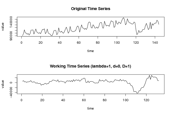
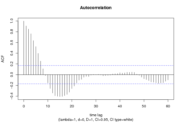
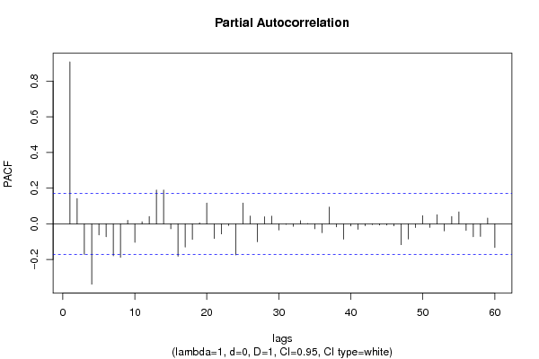
Title produced by software

(Partial) Autocorrelation Function

Date of computation

Tue, 20 Dec 2011 16:17:35 -0500

Cite this page as follows

Statistical Computations at FreeStatistics.org, Office for Research Development and Education, URL https://freestatistics.org/blog/index.php?v=date/2011/Dec/20/t1324415873guet9o5nfy6luhg.htm/, Retrieved Mon, 06 May 2024 04:03:30 +0000

Statistical Computations at FreeStatistics.org, Office for Research Development and Education, URL https://freestatistics.org/blog/index.php?pk=158275, Retrieved Mon, 06 May 2024 04:03:30 +0000

QR Codes:

Paste this QR Code to cite your computation.

Original text written by user:

IsPrivate?

No (this computation is public)

User-defined keywords

Estimated Impact

152

Family? (F = Feedback message, R = changed R code, M = changed R Module, P = changed Parameters, D = changed Data)

-     [Univariate Explorative Data Analysis] [Run Sequence gebo...] [2008-12-12 13:32:37] [76963dc1903f0f612b6153510a3818cf]
- R  D  [Univariate Explorative Data Analysis] [Run Sequence gebo...] [2008-12-17 12:14:40] [76963dc1903f0f612b6153510a3818cf]
-         [Univariate Explorative Data Analysis] [Run Sequence Plot...] [2008-12-22 18:19:51] [1ce0d16c8f4225c977b42c8fa93bc163]
- RMP       [Univariate Data Series] [Identifying Integ...] [2009-11-22 12:08:06] [b98453cac15ba1066b407e146608df68]
- RMP         [(Partial) Autocorrelation Function] [Births] [2010-11-29 09:36:27] [b98453cac15ba1066b407e146608df68]
- R PD          [(Partial) Autocorrelation Function] [WS9 3.1 ACF d=0, D=0] [2010-12-07 10:00:49] [afe9379cca749d06b3d6872e02cc47ed]
- R PD            [(Partial) Autocorrelation Function] [] [2011-12-04 10:34:49] [ec2187f7727da5d5d939740b21b8b68a]
-   PD                [(Partial) Autocorrelation Function] [] [2011-12-20 21:17:35] [542c32830549043c4555f1bd78aefedb] [Current]

Feedback Forum

Post a new message

Dataseries X:

Download CSV

Histogram

Boxplots

Summary of computational transaction
Raw Input	view raw input (R code)
Raw Output	view raw output of R engine
Computing time	1 seconds
R Server	'Gertrude Mary Cox' @ cox.wessa.net

\begin{tabular}{lllllllll}
\hline
Summary of computational transaction \tabularnewline
Raw Input & view raw input (R code)  \tabularnewline
Raw Output & view raw output of R engine  \tabularnewline
Computing time & 1 seconds \tabularnewline
R Server & 'Gertrude Mary Cox' @ cox.wessa.net \tabularnewline
\hline
\end{tabular}
%Source: https://freestatistics.org/blog/index.php?pk=158275&T=0

[TABLE]
[ROW][C]Summary of computational transaction[/C][/ROW]
[ROW][C]Raw Input[/C][C]view raw input (R code) [/C][/ROW]
[ROW][C]Raw Output[/C][C]view raw output of R engine [/C][/ROW]
[ROW][C]Computing time[/C][C]1 seconds[/C][/ROW]
[ROW][C]R Server[/C][C]'Gertrude Mary Cox' @ cox.wessa.net[/C][/ROW]
[/TABLE]
Source: https://freestatistics.org/blog/index.php?pk=158275&T=0

Globally Unique Identifier (entire table): ba.freestatistics.org/blog/index.php?pk=158275&T=0

As an alternative you can also use a QR Code:

The GUIDs for individual cells are displayed in the table below:

Summary of computational transaction
Raw Input	view raw input (R code)
Raw Output	view raw output of R engine
Computing time	1 seconds
R Server	'Gertrude Mary Cox' @ cox.wessa.net

Autocorrelation Function
Time lag k	ACF(k)	T-STAT	P-value
1	0.908595	10.439	0
2	0.850305	9.7693	0
3	0.762607	8.7617	0
4	0.635497	7.3013	0
5	0.524204	6.0226	0
6	0.397119	4.5625	6e-06
7	0.253637	2.9141	0.002096
8	0.11045	1.269	0.103341
9	-0.015398	-0.1769	0.429927
10	-0.152771	-1.7552	0.040772
11	-0.257294	-2.9561	0.001846
12	-0.341705	-3.9259	6.9e-05
13	-0.391895	-4.5025	7e-06
14	-0.402553	-4.625	4e-06
15	-0.407815	-4.6854	3e-06
16	-0.405046	-4.6536	4e-06
17	-0.389737	-4.4777	8e-06
18	-0.367821	-4.2259	2.2e-05
19	-0.326483	-3.751	0.000131
20	-0.258828	-2.9737	0.001749
21	-0.211602	-2.4311	0.008197
22	-0.154563	-1.7758	0.039036
23	-0.101041	-1.1609	0.123893
24	-0.087605	-1.0065	0.158008
25	-0.046674	-0.5362	0.296347
26	-0.031264	-0.3592	0.360012
27	-0.034084	-0.3916	0.347995
28	-0.008472	-0.0973	0.461302
29	0.004723	0.0543	0.478404
30	0.002705	0.0311	0.487628
31	0.006984	0.0802	0.468084
32	-0.004882	-0.0561	0.477677
33	-0.021483	-0.2468	0.402714
34	-0.016333	-0.1877	0.425719
35	-0.012652	-0.1454	0.442325
36	-0.008991	-0.1033	0.458939
37	0.015051	0.1729	0.431489
38	0.019118	0.2197	0.413241
39	0.022605	0.2597	0.397747
40	0.036211	0.416	0.339029
41	0.029456	0.3384	0.36779
42	0.034492	0.3963	0.346268
43	0.045395	0.5215	0.30143
44	0.043744	0.5026	0.308048
45	0.048274	0.5546	0.290046
46	0.043626	0.5012	0.308526
47	0.010506	0.1207	0.452055
48	-0.012409	-0.1426	0.443426
49	-0.045791	-0.5261	0.299853
50	-0.075945	-0.8725	0.192249
51	-0.091887	-1.0557	0.146517
52	-0.110592	-1.2706	0.103052
53	-0.136103	-1.5637	0.06014
54	-0.141592	-1.6268	0.053085
55	-0.150431	-1.7283	0.043135
56	-0.162487	-1.8668	0.032072
57	-0.153272	-1.761	0.04028
58	-0.149239	-1.7146	0.04438
59	-0.121979	-1.4014	0.081716
60	-0.09782	-1.1239	0.131554

\begin{tabular}{lllllllll}
\hline
Autocorrelation Function \tabularnewline
Time lag k & ACF(k) & T-STAT & P-value \tabularnewline
1 & 0.908595 & 10.439 & 0 \tabularnewline
2 & 0.850305 & 9.7693 & 0 \tabularnewline
3 & 0.762607 & 8.7617 & 0 \tabularnewline
4 & 0.635497 & 7.3013 & 0 \tabularnewline
5 & 0.524204 & 6.0226 & 0 \tabularnewline
6 & 0.397119 & 4.5625 & 6e-06 \tabularnewline
7 & 0.253637 & 2.9141 & 0.002096 \tabularnewline
8 & 0.11045 & 1.269 & 0.103341 \tabularnewline
9 & -0.015398 & -0.1769 & 0.429927 \tabularnewline
10 & -0.152771 & -1.7552 & 0.040772 \tabularnewline
11 & -0.257294 & -2.9561 & 0.001846 \tabularnewline
12 & -0.341705 & -3.9259 & 6.9e-05 \tabularnewline
13 & -0.391895 & -4.5025 & 7e-06 \tabularnewline
14 & -0.402553 & -4.625 & 4e-06 \tabularnewline
15 & -0.407815 & -4.6854 & 3e-06 \tabularnewline
16 & -0.405046 & -4.6536 & 4e-06 \tabularnewline
17 & -0.389737 & -4.4777 & 8e-06 \tabularnewline
18 & -0.367821 & -4.2259 & 2.2e-05 \tabularnewline
19 & -0.326483 & -3.751 & 0.000131 \tabularnewline
20 & -0.258828 & -2.9737 & 0.001749 \tabularnewline
21 & -0.211602 & -2.4311 & 0.008197 \tabularnewline
22 & -0.154563 & -1.7758 & 0.039036 \tabularnewline
23 & -0.101041 & -1.1609 & 0.123893 \tabularnewline
24 & -0.087605 & -1.0065 & 0.158008 \tabularnewline
25 & -0.046674 & -0.5362 & 0.296347 \tabularnewline
26 & -0.031264 & -0.3592 & 0.360012 \tabularnewline
27 & -0.034084 & -0.3916 & 0.347995 \tabularnewline
28 & -0.008472 & -0.0973 & 0.461302 \tabularnewline
29 & 0.004723 & 0.0543 & 0.478404 \tabularnewline
30 & 0.002705 & 0.0311 & 0.487628 \tabularnewline
31 & 0.006984 & 0.0802 & 0.468084 \tabularnewline
32 & -0.004882 & -0.0561 & 0.477677 \tabularnewline
33 & -0.021483 & -0.2468 & 0.402714 \tabularnewline
34 & -0.016333 & -0.1877 & 0.425719 \tabularnewline
35 & -0.012652 & -0.1454 & 0.442325 \tabularnewline
36 & -0.008991 & -0.1033 & 0.458939 \tabularnewline
37 & 0.015051 & 0.1729 & 0.431489 \tabularnewline
38 & 0.019118 & 0.2197 & 0.413241 \tabularnewline
39 & 0.022605 & 0.2597 & 0.397747 \tabularnewline
40 & 0.036211 & 0.416 & 0.339029 \tabularnewline
41 & 0.029456 & 0.3384 & 0.36779 \tabularnewline
42 & 0.034492 & 0.3963 & 0.346268 \tabularnewline
43 & 0.045395 & 0.5215 & 0.30143 \tabularnewline
44 & 0.043744 & 0.5026 & 0.308048 \tabularnewline
45 & 0.048274 & 0.5546 & 0.290046 \tabularnewline
46 & 0.043626 & 0.5012 & 0.308526 \tabularnewline
47 & 0.010506 & 0.1207 & 0.452055 \tabularnewline
48 & -0.012409 & -0.1426 & 0.443426 \tabularnewline
49 & -0.045791 & -0.5261 & 0.299853 \tabularnewline
50 & -0.075945 & -0.8725 & 0.192249 \tabularnewline
51 & -0.091887 & -1.0557 & 0.146517 \tabularnewline
52 & -0.110592 & -1.2706 & 0.103052 \tabularnewline
53 & -0.136103 & -1.5637 & 0.06014 \tabularnewline
54 & -0.141592 & -1.6268 & 0.053085 \tabularnewline
55 & -0.150431 & -1.7283 & 0.043135 \tabularnewline
56 & -0.162487 & -1.8668 & 0.032072 \tabularnewline
57 & -0.153272 & -1.761 & 0.04028 \tabularnewline
58 & -0.149239 & -1.7146 & 0.04438 \tabularnewline
59 & -0.121979 & -1.4014 & 0.081716 \tabularnewline
60 & -0.09782 & -1.1239 & 0.131554 \tabularnewline
\hline
\end{tabular}
%Source: https://freestatistics.org/blog/index.php?pk=158275&T=1

[TABLE]
[ROW][C]Autocorrelation Function[/C][/ROW]
[ROW][C]Time lag k[/C][C]ACF(k)[/C][C]T-STAT[/C][C]P-value[/C][/ROW]
[ROW][C]1[/C][C]0.908595[/C][C]10.439[/C][C]0[/C][/ROW]
[ROW][C]2[/C][C]0.850305[/C][C]9.7693[/C][C]0[/C][/ROW]
[ROW][C]3[/C][C]0.762607[/C][C]8.7617[/C][C]0[/C][/ROW]
[ROW][C]4[/C][C]0.635497[/C][C]7.3013[/C][C]0[/C][/ROW]
[ROW][C]5[/C][C]0.524204[/C][C]6.0226[/C][C]0[/C][/ROW]
[ROW][C]6[/C][C]0.397119[/C][C]4.5625[/C][C]6e-06[/C][/ROW]
[ROW][C]7[/C][C]0.253637[/C][C]2.9141[/C][C]0.002096[/C][/ROW]
[ROW][C]8[/C][C]0.11045[/C][C]1.269[/C][C]0.103341[/C][/ROW]
[ROW][C]9[/C][C]-0.015398[/C][C]-0.1769[/C][C]0.429927[/C][/ROW]
[ROW][C]10[/C][C]-0.152771[/C][C]-1.7552[/C][C]0.040772[/C][/ROW]
[ROW][C]11[/C][C]-0.257294[/C][C]-2.9561[/C][C]0.001846[/C][/ROW]
[ROW][C]12[/C][C]-0.341705[/C][C]-3.9259[/C][C]6.9e-05[/C][/ROW]
[ROW][C]13[/C][C]-0.391895[/C][C]-4.5025[/C][C]7e-06[/C][/ROW]
[ROW][C]14[/C][C]-0.402553[/C][C]-4.625[/C][C]4e-06[/C][/ROW]
[ROW][C]15[/C][C]-0.407815[/C][C]-4.6854[/C][C]3e-06[/C][/ROW]
[ROW][C]16[/C][C]-0.405046[/C][C]-4.6536[/C][C]4e-06[/C][/ROW]
[ROW][C]17[/C][C]-0.389737[/C][C]-4.4777[/C][C]8e-06[/C][/ROW]
[ROW][C]18[/C][C]-0.367821[/C][C]-4.2259[/C][C]2.2e-05[/C][/ROW]
[ROW][C]19[/C][C]-0.326483[/C][C]-3.751[/C][C]0.000131[/C][/ROW]
[ROW][C]20[/C][C]-0.258828[/C][C]-2.9737[/C][C]0.001749[/C][/ROW]
[ROW][C]21[/C][C]-0.211602[/C][C]-2.4311[/C][C]0.008197[/C][/ROW]
[ROW][C]22[/C][C]-0.154563[/C][C]-1.7758[/C][C]0.039036[/C][/ROW]
[ROW][C]23[/C][C]-0.101041[/C][C]-1.1609[/C][C]0.123893[/C][/ROW]
[ROW][C]24[/C][C]-0.087605[/C][C]-1.0065[/C][C]0.158008[/C][/ROW]
[ROW][C]25[/C][C]-0.046674[/C][C]-0.5362[/C][C]0.296347[/C][/ROW]
[ROW][C]26[/C][C]-0.031264[/C][C]-0.3592[/C][C]0.360012[/C][/ROW]
[ROW][C]27[/C][C]-0.034084[/C][C]-0.3916[/C][C]0.347995[/C][/ROW]
[ROW][C]28[/C][C]-0.008472[/C][C]-0.0973[/C][C]0.461302[/C][/ROW]
[ROW][C]29[/C][C]0.004723[/C][C]0.0543[/C][C]0.478404[/C][/ROW]
[ROW][C]30[/C][C]0.002705[/C][C]0.0311[/C][C]0.487628[/C][/ROW]
[ROW][C]31[/C][C]0.006984[/C][C]0.0802[/C][C]0.468084[/C][/ROW]
[ROW][C]32[/C][C]-0.004882[/C][C]-0.0561[/C][C]0.477677[/C][/ROW]
[ROW][C]33[/C][C]-0.021483[/C][C]-0.2468[/C][C]0.402714[/C][/ROW]
[ROW][C]34[/C][C]-0.016333[/C][C]-0.1877[/C][C]0.425719[/C][/ROW]
[ROW][C]35[/C][C]-0.012652[/C][C]-0.1454[/C][C]0.442325[/C][/ROW]
[ROW][C]36[/C][C]-0.008991[/C][C]-0.1033[/C][C]0.458939[/C][/ROW]
[ROW][C]37[/C][C]0.015051[/C][C]0.1729[/C][C]0.431489[/C][/ROW]
[ROW][C]38[/C][C]0.019118[/C][C]0.2197[/C][C]0.413241[/C][/ROW]
[ROW][C]39[/C][C]0.022605[/C][C]0.2597[/C][C]0.397747[/C][/ROW]
[ROW][C]40[/C][C]0.036211[/C][C]0.416[/C][C]0.339029[/C][/ROW]
[ROW][C]41[/C][C]0.029456[/C][C]0.3384[/C][C]0.36779[/C][/ROW]
[ROW][C]42[/C][C]0.034492[/C][C]0.3963[/C][C]0.346268[/C][/ROW]
[ROW][C]43[/C][C]0.045395[/C][C]0.5215[/C][C]0.30143[/C][/ROW]
[ROW][C]44[/C][C]0.043744[/C][C]0.5026[/C][C]0.308048[/C][/ROW]
[ROW][C]45[/C][C]0.048274[/C][C]0.5546[/C][C]0.290046[/C][/ROW]
[ROW][C]46[/C][C]0.043626[/C][C]0.5012[/C][C]0.308526[/C][/ROW]
[ROW][C]47[/C][C]0.010506[/C][C]0.1207[/C][C]0.452055[/C][/ROW]
[ROW][C]48[/C][C]-0.012409[/C][C]-0.1426[/C][C]0.443426[/C][/ROW]
[ROW][C]49[/C][C]-0.045791[/C][C]-0.5261[/C][C]0.299853[/C][/ROW]
[ROW][C]50[/C][C]-0.075945[/C][C]-0.8725[/C][C]0.192249[/C][/ROW]
[ROW][C]51[/C][C]-0.091887[/C][C]-1.0557[/C][C]0.146517[/C][/ROW]
[ROW][C]52[/C][C]-0.110592[/C][C]-1.2706[/C][C]0.103052[/C][/ROW]
[ROW][C]53[/C][C]-0.136103[/C][C]-1.5637[/C][C]0.06014[/C][/ROW]
[ROW][C]54[/C][C]-0.141592[/C][C]-1.6268[/C][C]0.053085[/C][/ROW]
[ROW][C]55[/C][C]-0.150431[/C][C]-1.7283[/C][C]0.043135[/C][/ROW]
[ROW][C]56[/C][C]-0.162487[/C][C]-1.8668[/C][C]0.032072[/C][/ROW]
[ROW][C]57[/C][C]-0.153272[/C][C]-1.761[/C][C]0.04028[/C][/ROW]
[ROW][C]58[/C][C]-0.149239[/C][C]-1.7146[/C][C]0.04438[/C][/ROW]
[ROW][C]59[/C][C]-0.121979[/C][C]-1.4014[/C][C]0.081716[/C][/ROW]
[ROW][C]60[/C][C]-0.09782[/C][C]-1.1239[/C][C]0.131554[/C][/ROW]
[/TABLE]
Source: https://freestatistics.org/blog/index.php?pk=158275&T=1

Globally Unique Identifier (entire table): ba.freestatistics.org/blog/index.php?pk=158275&T=1

As an alternative you can also use a QR Code:

The GUIDs for individual cells are displayed in the table below:

Autocorrelation Function
Time lag k	ACF(k)	T-STAT	P-value
1	0.908595	10.439	0
2	0.850305	9.7693	0
3	0.762607	8.7617	0
4	0.635497	7.3013	0
5	0.524204	6.0226	0
6	0.397119	4.5625	6e-06
7	0.253637	2.9141	0.002096
8	0.11045	1.269	0.103341
9	-0.015398	-0.1769	0.429927
10	-0.152771	-1.7552	0.040772
11	-0.257294	-2.9561	0.001846
12	-0.341705	-3.9259	6.9e-05
13	-0.391895	-4.5025	7e-06
14	-0.402553	-4.625	4e-06
15	-0.407815	-4.6854	3e-06
16	-0.405046	-4.6536	4e-06
17	-0.389737	-4.4777	8e-06
18	-0.367821	-4.2259	2.2e-05
19	-0.326483	-3.751	0.000131
20	-0.258828	-2.9737	0.001749
21	-0.211602	-2.4311	0.008197
22	-0.154563	-1.7758	0.039036
23	-0.101041	-1.1609	0.123893
24	-0.087605	-1.0065	0.158008
25	-0.046674	-0.5362	0.296347
26	-0.031264	-0.3592	0.360012
27	-0.034084	-0.3916	0.347995
28	-0.008472	-0.0973	0.461302
29	0.004723	0.0543	0.478404
30	0.002705	0.0311	0.487628
31	0.006984	0.0802	0.468084
32	-0.004882	-0.0561	0.477677
33	-0.021483	-0.2468	0.402714
34	-0.016333	-0.1877	0.425719
35	-0.012652	-0.1454	0.442325
36	-0.008991	-0.1033	0.458939
37	0.015051	0.1729	0.431489
38	0.019118	0.2197	0.413241
39	0.022605	0.2597	0.397747
40	0.036211	0.416	0.339029
41	0.029456	0.3384	0.36779
42	0.034492	0.3963	0.346268
43	0.045395	0.5215	0.30143
44	0.043744	0.5026	0.308048
45	0.048274	0.5546	0.290046
46	0.043626	0.5012	0.308526
47	0.010506	0.1207	0.452055
48	-0.012409	-0.1426	0.443426
49	-0.045791	-0.5261	0.299853
50	-0.075945	-0.8725	0.192249
51	-0.091887	-1.0557	0.146517
52	-0.110592	-1.2706	0.103052
53	-0.136103	-1.5637	0.06014
54	-0.141592	-1.6268	0.053085
55	-0.150431	-1.7283	0.043135
56	-0.162487	-1.8668	0.032072
57	-0.153272	-1.761	0.04028
58	-0.149239	-1.7146	0.04438
59	-0.121979	-1.4014	0.081716
60	-0.09782	-1.1239	0.131554

Partial Autocorrelation Function
Time lag k	PACF(k)	T-STAT	P-value
1	0.908595	10.439	0
2	0.141926	1.6306	0.052678
3	-0.171291	-1.968	0.025583
4	-0.33873	-3.8917	7.9e-05
5	-0.062692	-0.7203	0.236313
6	-0.072527	-0.8333	0.203097
7	-0.179223	-2.0591	0.020725
8	-0.187891	-2.1587	0.016341
9	0.019551	0.2246	0.41131
10	-0.104156	-1.1967	0.116793
11	0.011366	0.1306	0.44815
12	0.040762	0.4683	0.320164
13	0.1899	2.1818	0.015448
14	0.189532	2.1776	0.015608
15	-0.027897	-0.3205	0.374542
16	-0.182261	-2.094	0.019085
17	-0.130435	-1.4986	0.068185
18	-0.087224	-1.0021	0.159058
19	0.006083	0.0699	0.472193
20	0.116479	1.3382	0.09156
21	-0.082688	-0.95	0.171922
22	-0.056668	-0.6511	0.258068
23	-0.009846	-0.1131	0.455053
24	-0.174682	-2.0069	0.023399
25	0.116398	1.3373	0.091711
26	0.043701	0.5021	0.308222
27	-0.100804	-1.1582	0.124447
28	0.039435	0.4531	0.325619
29	0.042804	0.4918	0.311846
30	-0.034824	-0.4001	0.344867
31	-0.003133	-0.036	0.485669
32	-0.013855	-0.1592	0.436884
33	0.01756	0.2017	0.420212
34	0.000699	0.008	0.496802
35	-0.027754	-0.3189	0.375166
36	-0.049884	-0.5731	0.283767
37	0.094245	1.0828	0.140438
38	-0.016733	-0.1923	0.42392
39	-0.086392	-0.9926	0.161369
40	-0.011562	-0.1328	0.447264
41	-0.030657	-0.3522	0.362617
42	-0.010277	-0.1181	0.453097
43	-0.004122	-0.0474	0.481147
44	-0.007015	-0.0806	0.467943
45	-0.006602	-0.0759	0.469826
46	-0.011308	-0.1299	0.448413
47	-0.11711	-1.3455	0.090387
48	-0.084872	-0.9751	0.165645
49	-0.020627	-0.237	0.406518
50	0.045592	0.5238	0.300642
51	-0.020093	-0.2309	0.408893
52	0.050789	0.5835	0.280268
53	-0.039392	-0.4526	0.325795
54	0.041194	0.4733	0.318398
55	0.066872	0.7683	0.22184
56	-0.036945	-0.4245	0.335958
57	-0.072734	-0.8357	0.20243
58	-0.070633	-0.8115	0.209267
59	0.032222	0.3702	0.355911
60	-0.132794	-1.5257	0.06474

\begin{tabular}{lllllllll}
\hline
Partial Autocorrelation Function \tabularnewline
Time lag k & PACF(k) & T-STAT & P-value \tabularnewline
1 & 0.908595 & 10.439 & 0 \tabularnewline
2 & 0.141926 & 1.6306 & 0.052678 \tabularnewline
3 & -0.171291 & -1.968 & 0.025583 \tabularnewline
4 & -0.33873 & -3.8917 & 7.9e-05 \tabularnewline
5 & -0.062692 & -0.7203 & 0.236313 \tabularnewline
6 & -0.072527 & -0.8333 & 0.203097 \tabularnewline
7 & -0.179223 & -2.0591 & 0.020725 \tabularnewline
8 & -0.187891 & -2.1587 & 0.016341 \tabularnewline
9 & 0.019551 & 0.2246 & 0.41131 \tabularnewline
10 & -0.104156 & -1.1967 & 0.116793 \tabularnewline
11 & 0.011366 & 0.1306 & 0.44815 \tabularnewline
12 & 0.040762 & 0.4683 & 0.320164 \tabularnewline
13 & 0.1899 & 2.1818 & 0.015448 \tabularnewline
14 & 0.189532 & 2.1776 & 0.015608 \tabularnewline
15 & -0.027897 & -0.3205 & 0.374542 \tabularnewline
16 & -0.182261 & -2.094 & 0.019085 \tabularnewline
17 & -0.130435 & -1.4986 & 0.068185 \tabularnewline
18 & -0.087224 & -1.0021 & 0.159058 \tabularnewline
19 & 0.006083 & 0.0699 & 0.472193 \tabularnewline
20 & 0.116479 & 1.3382 & 0.09156 \tabularnewline
21 & -0.082688 & -0.95 & 0.171922 \tabularnewline
22 & -0.056668 & -0.6511 & 0.258068 \tabularnewline
23 & -0.009846 & -0.1131 & 0.455053 \tabularnewline
24 & -0.174682 & -2.0069 & 0.023399 \tabularnewline
25 & 0.116398 & 1.3373 & 0.091711 \tabularnewline
26 & 0.043701 & 0.5021 & 0.308222 \tabularnewline
27 & -0.100804 & -1.1582 & 0.124447 \tabularnewline
28 & 0.039435 & 0.4531 & 0.325619 \tabularnewline
29 & 0.042804 & 0.4918 & 0.311846 \tabularnewline
30 & -0.034824 & -0.4001 & 0.344867 \tabularnewline
31 & -0.003133 & -0.036 & 0.485669 \tabularnewline
32 & -0.013855 & -0.1592 & 0.436884 \tabularnewline
33 & 0.01756 & 0.2017 & 0.420212 \tabularnewline
34 & 0.000699 & 0.008 & 0.496802 \tabularnewline
35 & -0.027754 & -0.3189 & 0.375166 \tabularnewline
36 & -0.049884 & -0.5731 & 0.283767 \tabularnewline
37 & 0.094245 & 1.0828 & 0.140438 \tabularnewline
38 & -0.016733 & -0.1923 & 0.42392 \tabularnewline
39 & -0.086392 & -0.9926 & 0.161369 \tabularnewline
40 & -0.011562 & -0.1328 & 0.447264 \tabularnewline
41 & -0.030657 & -0.3522 & 0.362617 \tabularnewline
42 & -0.010277 & -0.1181 & 0.453097 \tabularnewline
43 & -0.004122 & -0.0474 & 0.481147 \tabularnewline
44 & -0.007015 & -0.0806 & 0.467943 \tabularnewline
45 & -0.006602 & -0.0759 & 0.469826 \tabularnewline
46 & -0.011308 & -0.1299 & 0.448413 \tabularnewline
47 & -0.11711 & -1.3455 & 0.090387 \tabularnewline
48 & -0.084872 & -0.9751 & 0.165645 \tabularnewline
49 & -0.020627 & -0.237 & 0.406518 \tabularnewline
50 & 0.045592 & 0.5238 & 0.300642 \tabularnewline
51 & -0.020093 & -0.2309 & 0.408893 \tabularnewline
52 & 0.050789 & 0.5835 & 0.280268 \tabularnewline
53 & -0.039392 & -0.4526 & 0.325795 \tabularnewline
54 & 0.041194 & 0.4733 & 0.318398 \tabularnewline
55 & 0.066872 & 0.7683 & 0.22184 \tabularnewline
56 & -0.036945 & -0.4245 & 0.335958 \tabularnewline
57 & -0.072734 & -0.8357 & 0.20243 \tabularnewline
58 & -0.070633 & -0.8115 & 0.209267 \tabularnewline
59 & 0.032222 & 0.3702 & 0.355911 \tabularnewline
60 & -0.132794 & -1.5257 & 0.06474 \tabularnewline
\hline
\end{tabular}
%Source: https://freestatistics.org/blog/index.php?pk=158275&T=2

[TABLE]
[ROW][C]Partial Autocorrelation Function[/C][/ROW]
[ROW][C]Time lag k[/C][C]PACF(k)[/C][C]T-STAT[/C][C]P-value[/C][/ROW]
[ROW][C]1[/C][C]0.908595[/C][C]10.439[/C][C]0[/C][/ROW]
[ROW][C]2[/C][C]0.141926[/C][C]1.6306[/C][C]0.052678[/C][/ROW]
[ROW][C]3[/C][C]-0.171291[/C][C]-1.968[/C][C]0.025583[/C][/ROW]
[ROW][C]4[/C][C]-0.33873[/C][C]-3.8917[/C][C]7.9e-05[/C][/ROW]
[ROW][C]5[/C][C]-0.062692[/C][C]-0.7203[/C][C]0.236313[/C][/ROW]
[ROW][C]6[/C][C]-0.072527[/C][C]-0.8333[/C][C]0.203097[/C][/ROW]
[ROW][C]7[/C][C]-0.179223[/C][C]-2.0591[/C][C]0.020725[/C][/ROW]
[ROW][C]8[/C][C]-0.187891[/C][C]-2.1587[/C][C]0.016341[/C][/ROW]
[ROW][C]9[/C][C]0.019551[/C][C]0.2246[/C][C]0.41131[/C][/ROW]
[ROW][C]10[/C][C]-0.104156[/C][C]-1.1967[/C][C]0.116793[/C][/ROW]
[ROW][C]11[/C][C]0.011366[/C][C]0.1306[/C][C]0.44815[/C][/ROW]
[ROW][C]12[/C][C]0.040762[/C][C]0.4683[/C][C]0.320164[/C][/ROW]
[ROW][C]13[/C][C]0.1899[/C][C]2.1818[/C][C]0.015448[/C][/ROW]
[ROW][C]14[/C][C]0.189532[/C][C]2.1776[/C][C]0.015608[/C][/ROW]
[ROW][C]15[/C][C]-0.027897[/C][C]-0.3205[/C][C]0.374542[/C][/ROW]
[ROW][C]16[/C][C]-0.182261[/C][C]-2.094[/C][C]0.019085[/C][/ROW]
[ROW][C]17[/C][C]-0.130435[/C][C]-1.4986[/C][C]0.068185[/C][/ROW]
[ROW][C]18[/C][C]-0.087224[/C][C]-1.0021[/C][C]0.159058[/C][/ROW]
[ROW][C]19[/C][C]0.006083[/C][C]0.0699[/C][C]0.472193[/C][/ROW]
[ROW][C]20[/C][C]0.116479[/C][C]1.3382[/C][C]0.09156[/C][/ROW]
[ROW][C]21[/C][C]-0.082688[/C][C]-0.95[/C][C]0.171922[/C][/ROW]
[ROW][C]22[/C][C]-0.056668[/C][C]-0.6511[/C][C]0.258068[/C][/ROW]
[ROW][C]23[/C][C]-0.009846[/C][C]-0.1131[/C][C]0.455053[/C][/ROW]
[ROW][C]24[/C][C]-0.174682[/C][C]-2.0069[/C][C]0.023399[/C][/ROW]
[ROW][C]25[/C][C]0.116398[/C][C]1.3373[/C][C]0.091711[/C][/ROW]
[ROW][C]26[/C][C]0.043701[/C][C]0.5021[/C][C]0.308222[/C][/ROW]
[ROW][C]27[/C][C]-0.100804[/C][C]-1.1582[/C][C]0.124447[/C][/ROW]
[ROW][C]28[/C][C]0.039435[/C][C]0.4531[/C][C]0.325619[/C][/ROW]
[ROW][C]29[/C][C]0.042804[/C][C]0.4918[/C][C]0.311846[/C][/ROW]
[ROW][C]30[/C][C]-0.034824[/C][C]-0.4001[/C][C]0.344867[/C][/ROW]
[ROW][C]31[/C][C]-0.003133[/C][C]-0.036[/C][C]0.485669[/C][/ROW]
[ROW][C]32[/C][C]-0.013855[/C][C]-0.1592[/C][C]0.436884[/C][/ROW]
[ROW][C]33[/C][C]0.01756[/C][C]0.2017[/C][C]0.420212[/C][/ROW]
[ROW][C]34[/C][C]0.000699[/C][C]0.008[/C][C]0.496802[/C][/ROW]
[ROW][C]35[/C][C]-0.027754[/C][C]-0.3189[/C][C]0.375166[/C][/ROW]
[ROW][C]36[/C][C]-0.049884[/C][C]-0.5731[/C][C]0.283767[/C][/ROW]
[ROW][C]37[/C][C]0.094245[/C][C]1.0828[/C][C]0.140438[/C][/ROW]
[ROW][C]38[/C][C]-0.016733[/C][C]-0.1923[/C][C]0.42392[/C][/ROW]
[ROW][C]39[/C][C]-0.086392[/C][C]-0.9926[/C][C]0.161369[/C][/ROW]
[ROW][C]40[/C][C]-0.011562[/C][C]-0.1328[/C][C]0.447264[/C][/ROW]
[ROW][C]41[/C][C]-0.030657[/C][C]-0.3522[/C][C]0.362617[/C][/ROW]
[ROW][C]42[/C][C]-0.010277[/C][C]-0.1181[/C][C]0.453097[/C][/ROW]
[ROW][C]43[/C][C]-0.004122[/C][C]-0.0474[/C][C]0.481147[/C][/ROW]
[ROW][C]44[/C][C]-0.007015[/C][C]-0.0806[/C][C]0.467943[/C][/ROW]
[ROW][C]45[/C][C]-0.006602[/C][C]-0.0759[/C][C]0.469826[/C][/ROW]
[ROW][C]46[/C][C]-0.011308[/C][C]-0.1299[/C][C]0.448413[/C][/ROW]
[ROW][C]47[/C][C]-0.11711[/C][C]-1.3455[/C][C]0.090387[/C][/ROW]
[ROW][C]48[/C][C]-0.084872[/C][C]-0.9751[/C][C]0.165645[/C][/ROW]
[ROW][C]49[/C][C]-0.020627[/C][C]-0.237[/C][C]0.406518[/C][/ROW]
[ROW][C]50[/C][C]0.045592[/C][C]0.5238[/C][C]0.300642[/C][/ROW]
[ROW][C]51[/C][C]-0.020093[/C][C]-0.2309[/C][C]0.408893[/C][/ROW]
[ROW][C]52[/C][C]0.050789[/C][C]0.5835[/C][C]0.280268[/C][/ROW]
[ROW][C]53[/C][C]-0.039392[/C][C]-0.4526[/C][C]0.325795[/C][/ROW]
[ROW][C]54[/C][C]0.041194[/C][C]0.4733[/C][C]0.318398[/C][/ROW]
[ROW][C]55[/C][C]0.066872[/C][C]0.7683[/C][C]0.22184[/C][/ROW]
[ROW][C]56[/C][C]-0.036945[/C][C]-0.4245[/C][C]0.335958[/C][/ROW]
[ROW][C]57[/C][C]-0.072734[/C][C]-0.8357[/C][C]0.20243[/C][/ROW]
[ROW][C]58[/C][C]-0.070633[/C][C]-0.8115[/C][C]0.209267[/C][/ROW]
[ROW][C]59[/C][C]0.032222[/C][C]0.3702[/C][C]0.355911[/C][/ROW]
[ROW][C]60[/C][C]-0.132794[/C][C]-1.5257[/C][C]0.06474[/C][/ROW]
[/TABLE]
Source: https://freestatistics.org/blog/index.php?pk=158275&T=2

Globally Unique Identifier (entire table): ba.freestatistics.org/blog/index.php?pk=158275&T=2

As an alternative you can also use a QR Code:

The GUIDs for individual cells are displayed in the table below:

Partial Autocorrelation Function
Time lag k	PACF(k)	T-STAT	P-value
1	0.908595	10.439	0
2	0.141926	1.6306	0.052678
3	-0.171291	-1.968	0.025583
4	-0.33873	-3.8917	7.9e-05
5	-0.062692	-0.7203	0.236313
6	-0.072527	-0.8333	0.203097
7	-0.179223	-2.0591	0.020725
8	-0.187891	-2.1587	0.016341
9	0.019551	0.2246	0.41131
10	-0.104156	-1.1967	0.116793
11	0.011366	0.1306	0.44815
12	0.040762	0.4683	0.320164
13	0.1899	2.1818	0.015448
14	0.189532	2.1776	0.015608
15	-0.027897	-0.3205	0.374542
16	-0.182261	-2.094	0.019085
17	-0.130435	-1.4986	0.068185
18	-0.087224	-1.0021	0.159058
19	0.006083	0.0699	0.472193
20	0.116479	1.3382	0.09156
21	-0.082688	-0.95	0.171922
22	-0.056668	-0.6511	0.258068
23	-0.009846	-0.1131	0.455053
24	-0.174682	-2.0069	0.023399
25	0.116398	1.3373	0.091711
26	0.043701	0.5021	0.308222
27	-0.100804	-1.1582	0.124447
28	0.039435	0.4531	0.325619
29	0.042804	0.4918	0.311846
30	-0.034824	-0.4001	0.344867
31	-0.003133	-0.036	0.485669
32	-0.013855	-0.1592	0.436884
33	0.01756	0.2017	0.420212
34	0.000699	0.008	0.496802
35	-0.027754	-0.3189	0.375166
36	-0.049884	-0.5731	0.283767
37	0.094245	1.0828	0.140438
38	-0.016733	-0.1923	0.42392
39	-0.086392	-0.9926	0.161369
40	-0.011562	-0.1328	0.447264
41	-0.030657	-0.3522	0.362617
42	-0.010277	-0.1181	0.453097
43	-0.004122	-0.0474	0.481147
44	-0.007015	-0.0806	0.467943
45	-0.006602	-0.0759	0.469826
46	-0.011308	-0.1299	0.448413
47	-0.11711	-1.3455	0.090387
48	-0.084872	-0.9751	0.165645
49	-0.020627	-0.237	0.406518
50	0.045592	0.5238	0.300642
51	-0.020093	-0.2309	0.408893
52	0.050789	0.5835	0.280268
53	-0.039392	-0.4526	0.325795
54	0.041194	0.4733	0.318398
55	0.066872	0.7683	0.22184
56	-0.036945	-0.4245	0.335958
57	-0.072734	-0.8357	0.20243
58	-0.070633	-0.8115	0.209267
59	0.032222	0.3702	0.355911
60	-0.132794	-1.5257	0.06474

Figure 1

PNG link

Postscript link

PDF link

Figure 2

PNG link

Postscript link

PDF link

Figure 3

PNG link

Postscript link

PDF link

Parameters (Session):

par1 = 4 ; par2 = Include Monthly Dummies ; par3 = No Linear Trend ;

Parameters (R input):

par1 = 60 ; par2 = 1 ; par3 = 0 ; par4 = 1 ; par5 = 12 ; par6 = White Noise ; par7 = 0.95 ; par8 = ;

R code (references can be found in the software module):

if (par1 == 'Default') {
par1 = 10*log10(length(x))
} else {
par1 <- as.numeric(par1)
}
par2 <- as.numeric(par2)
par3 <- as.numeric(par3)
par4 <- as.numeric(par4)
par5 <- as.numeric(par5)
if (par6 == 'White Noise') par6 <- 'white' else par6 <- 'ma'
par7 <- as.numeric(par7)
if (par8 != '') par8 <- as.numeric(par8)
ox <- x
if (par8 == '') {
if (par2 == 0) {
x <- log(x)
} else {
x <- (x ^ par2 - 1) / par2
}
} else {
x <- log(x,base=par8)
}
if (par3 > 0) x <- diff(x,lag=1,difference=par3)
if (par4 > 0) x <- diff(x,lag=par5,difference=par4)
bitmap(file='picts.png')
op <- par(mfrow=c(2,1))
plot(ox,type='l',main='Original Time Series',xlab='time',ylab='value')
if (par8=='') {
mytitle <- paste('Working Time Series (lambda=',par2,', d=',par3,', D=',par4,')',sep='')
mysub <- paste('(lambda=',par2,', d=',par3,', D=',par4,', CI=', par7, ', CI type=',par6,')',sep='')
} else {
mytitle <- paste('Working Time Series (base=',par8,', d=',par3,', D=',par4,')',sep='')
mysub <- paste('(base=',par8,', d=',par3,', D=',par4,', CI=', par7, ', CI type=',par6,')',sep='')
}
plot(x,type='l', main=mytitle,xlab='time',ylab='value')
par(op)
dev.off()
bitmap(file='pic1.png')
racf <- acf(x, par1, main='Autocorrelation', xlab='time lag', ylab='ACF', ci.type=par6, ci=par7, sub=mysub)
dev.off()
bitmap(file='pic2.png')
rpacf <- pacf(x,par1,main='Partial Autocorrelation',xlab='lags',ylab='PACF',sub=mysub)
dev.off()
(myacf <- c(racf$acf))
(mypacf <- c(rpacf$acf))
lengthx <- length(x)
sqrtn <- sqrt(lengthx)
load(file='createtable')
a<-table.start()
a<-table.row.start(a)
a<-table.element(a,'Autocorrelation Function',4,TRUE)
a<-table.row.end(a)
a<-table.row.start(a)
a<-table.element(a,'Time lag k',header=TRUE)
a<-table.element(a,hyperlink('basics.htm','ACF(k)','click here for more information about the Autocorrelation Function'),header=TRUE)
a<-table.element(a,'T-STAT',header=TRUE)
a<-table.element(a,'P-value',header=TRUE)
a<-table.row.end(a)
for (i in 2:(par1+1)) {
a<-table.row.start(a)
a<-table.element(a,i-1,header=TRUE)
a<-table.element(a,round(myacf[i],6))
mytstat <- myacf[i]*sqrtn
a<-table.element(a,round(mytstat,4))
a<-table.element(a,round(1-pt(abs(mytstat),lengthx),6))
a<-table.row.end(a)
}
a<-table.end(a)
table.save(a,file='mytable.tab')
a<-table.start()
a<-table.row.start(a)
a<-table.element(a,'Partial Autocorrelation Function',4,TRUE)
a<-table.row.end(a)
a<-table.row.start(a)
a<-table.element(a,'Time lag k',header=TRUE)
a<-table.element(a,hyperlink('basics.htm','PACF(k)','click here for more information about the Partial Autocorrelation Function'),header=TRUE)
a<-table.element(a,'T-STAT',header=TRUE)
a<-table.element(a,'P-value',header=TRUE)
a<-table.row.end(a)
for (i in 1:par1) {
a<-table.row.start(a)
a<-table.element(a,i,header=TRUE)
a<-table.element(a,round(mypacf[i],6))
mytstat <- mypacf[i]*sqrtn
a<-table.element(a,round(mytstat,4))
a<-table.element(a,round(1-pt(abs(mytstat),lengthx),6))
a<-table.row.end(a)
}
a<-table.end(a)
table.save(a,file='mytable1.tab')

Free Statistics

Description of Statistical Computation

Tree of Dependent Computations

Dataset

Tables (Output of Computation)

Figures (Output of Computation)

Input Parameters & R Code