Free Statistics
of Irreproducible Research!
Description of Statistical Computation | |||||||||||||||||||||
|---|---|---|---|---|---|---|---|---|---|---|---|---|---|---|---|---|---|---|---|---|---|
| Author's title | |||||||||||||||||||||
| Author | *The author of this computation has been verified* | ||||||||||||||||||||
| R Software Module | rwasp_meanplot.wasp | ||||||||||||||||||||
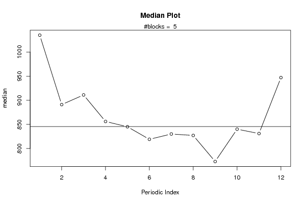
| Title produced by software | Mean Plot | ||||||||||||||||||||
| Date of computation | Tue, 20 Dec 2011 15:04:13 -0500 | ||||||||||||||||||||
| Cite this page as follows | Statistical Computations at FreeStatistics.org, Office for Research Development and Education, URL https://freestatistics.org/blog/index.php?v=date/2011/Dec/20/t1324411468et5p9oyyx52k5jt.htm/, Retrieved Mon, 06 May 2024 02:33:26 +0000 | ||||||||||||||||||||
| Statistical Computations at FreeStatistics.org, Office for Research Development and Education, URL https://freestatistics.org/blog/index.php?pk=158218, Retrieved Mon, 06 May 2024 02:33:26 +0000 | |||||||||||||||||||||
| QR Codes: | |||||||||||||||||||||
|
| |||||||||||||||||||||
| Original text written by user: | |||||||||||||||||||||
| IsPrivate? | No (this computation is public) | ||||||||||||||||||||
| User-defined keywords | |||||||||||||||||||||
| Estimated Impact | 99 | ||||||||||||||||||||
Tree of Dependent Computations | |||||||||||||||||||||
| Family? (F = Feedback message, R = changed R code, M = changed R Module, P = changed Parameters, D = changed Data) | |||||||||||||||||||||
| - [Univariate Data Series] [Arabica Price in ...] [2008-01-05 23:14:31] [74be16979710d4c4e7c6647856088456] - RMPD [Univariate Data Series] [Workshop 6 - Mini...] [2011-11-15 16:41:21] [74be16979710d4c4e7c6647856088456] - RMPD [Central Tendency] [tut2] [2011-11-15 20:51:03] [f7a862281046b7153543b12c78921b36] - RMPD [Mean Plot] [paper26] [2011-12-20 20:04:13] [47995d3a8fac585eeb070a274b466f8c] [Current] | |||||||||||||||||||||
| Feedback Forum | |||||||||||||||||||||
Post a new message | |||||||||||||||||||||
Dataset | |||||||||||||||||||||
| Dataseries X: | |||||||||||||||||||||
1200 916 878 841 824 819 823 825 773 836 862 886 1010 846 911 856 881 830 830 827 773 797 826 947 1110 896 917 873 845 807 841 829 781 861 831 969 991 891 945 911 847 823 838 862 822 864 862 1044 1035 858 889 832 810 792 812 783 773 840 820 945 | |||||||||||||||||||||
Tables (Output of Computation) | |||||||||||||||||||||
| |||||||||||||||||||||
Figures (Output of Computation) | |||||||||||||||||||||
Input Parameters & R Code | |||||||||||||||||||||
| Parameters (Session): | |||||||||||||||||||||
| par1 = 12 ; | |||||||||||||||||||||
| Parameters (R input): | |||||||||||||||||||||
| par1 = 12 ; | |||||||||||||||||||||
| R code (references can be found in the software module): | |||||||||||||||||||||
par1 <- as.numeric(par1) | |||||||||||||||||||||