Free Statistics
of Irreproducible Research!
Description of Statistical Computation | |||||||||||||||||||||||||||||||||||||||||||||||||||||
|---|---|---|---|---|---|---|---|---|---|---|---|---|---|---|---|---|---|---|---|---|---|---|---|---|---|---|---|---|---|---|---|---|---|---|---|---|---|---|---|---|---|---|---|---|---|---|---|---|---|---|---|---|---|
| Author's title | |||||||||||||||||||||||||||||||||||||||||||||||||||||
| Author | *The author of this computation has been verified* | ||||||||||||||||||||||||||||||||||||||||||||||||||||
| R Software Module | rwasp_edauni.wasp | ||||||||||||||||||||||||||||||||||||||||||||||||||||
| Title produced by software | Univariate Explorative Data Analysis | ||||||||||||||||||||||||||||||||||||||||||||||||||||
| Date of computation | Fri, 16 Dec 2011 10:55:55 -0500 | ||||||||||||||||||||||||||||||||||||||||||||||||||||
| Cite this page as follows | Statistical Computations at FreeStatistics.org, Office for Research Development and Education, URL https://freestatistics.org/blog/index.php?v=date/2011/Dec/16/t1324051009c965r0t39lc633d.htm/, Retrieved Sun, 05 May 2024 15:57:55 +0000 | ||||||||||||||||||||||||||||||||||||||||||||||||||||
| Statistical Computations at FreeStatistics.org, Office for Research Development and Education, URL https://freestatistics.org/blog/index.php?pk=156068, Retrieved Sun, 05 May 2024 15:57:55 +0000 | |||||||||||||||||||||||||||||||||||||||||||||||||||||
| QR Codes: | |||||||||||||||||||||||||||||||||||||||||||||||||||||
|
| |||||||||||||||||||||||||||||||||||||||||||||||||||||
| Original text written by user: | |||||||||||||||||||||||||||||||||||||||||||||||||||||
| IsPrivate? | No (this computation is public) | ||||||||||||||||||||||||||||||||||||||||||||||||||||
| User-defined keywords | |||||||||||||||||||||||||||||||||||||||||||||||||||||
| Estimated Impact | 113 | ||||||||||||||||||||||||||||||||||||||||||||||||||||
Tree of Dependent Computations | |||||||||||||||||||||||||||||||||||||||||||||||||||||
| Family? (F = Feedback message, R = changed R code, M = changed R Module, P = changed Parameters, D = changed Data) | |||||||||||||||||||||||||||||||||||||||||||||||||||||
| - [Histogram] [Workshop 1 - Task 1] [2011-10-03 18:33:04] [fbaf17a8836493f6de0f4e0e997711e1] - RMPD [Univariate Data Series] [Paper run sequenc...] [2011-12-15 17:43:06] [abc1cbe561c2c4615f632bb3153b1275] - RMP [Univariate Explorative Data Analysis] [Paper Univariate Eda] [2011-12-16 15:55:55] [c98b04636162cea751932dfe577607eb] [Current] - RMP [ARIMA Backward Selection] [Paper ARIMA Backw...] [2011-12-23 14:17:11] [abc1cbe561c2c4615f632bb3153b1275] - RMP [ARIMA Backward Selection] [ARIMA Backward Se...] [2011-12-23 14:21:51] [abc1cbe561c2c4615f632bb3153b1275] | |||||||||||||||||||||||||||||||||||||||||||||||||||||
| Feedback Forum | |||||||||||||||||||||||||||||||||||||||||||||||||||||
Post a new message | |||||||||||||||||||||||||||||||||||||||||||||||||||||
Dataset | |||||||||||||||||||||||||||||||||||||||||||||||||||||
| Dataseries X: | |||||||||||||||||||||||||||||||||||||||||||||||||||||
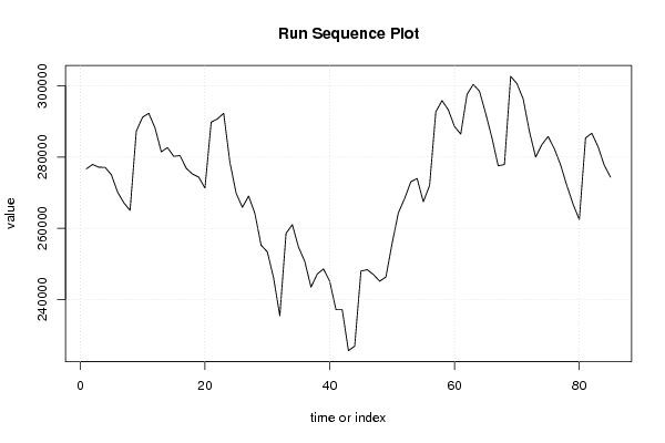
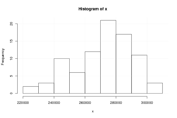
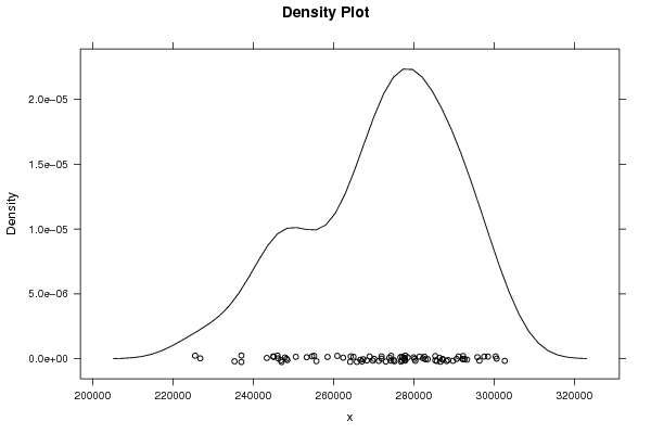
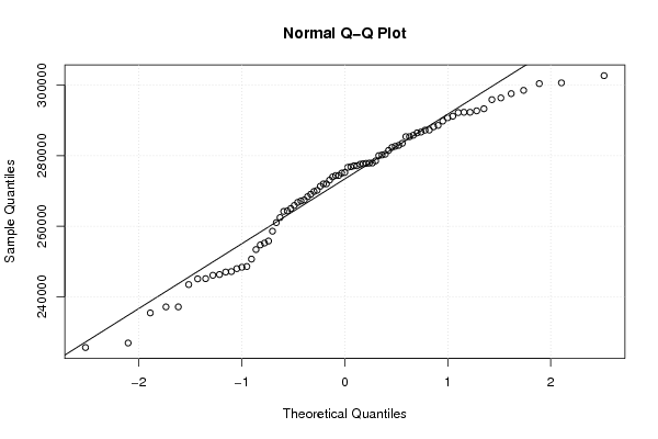
276687 277915 277128 277103 275037 270150 267140 264993 287259 291186 292300 288186 281477 282656 280190 280408 276836 275216 274352 271311 289802 290726 292300 278506 269826 265861 269034 264176 255198 253353 246057 235372 258556 260993 254663 250643 243422 247105 248541 245039 237080 237085 225554 226839 247934 248333 246969 245098 246263 255765 264319 268347 273046 273963 267430 271993 292710 295881 293299 288576 286445 297584 300431 298522 292213 285383 277537 277891 302686 300653 296369 287224 279998 283495 285775 282329 277799 271980 266730 262433 285378 286692 282917 277686 274371 | |||||||||||||||||||||||||||||||||||||||||||||||||||||
Tables (Output of Computation) | |||||||||||||||||||||||||||||||||||||||||||||||||||||
| |||||||||||||||||||||||||||||||||||||||||||||||||||||
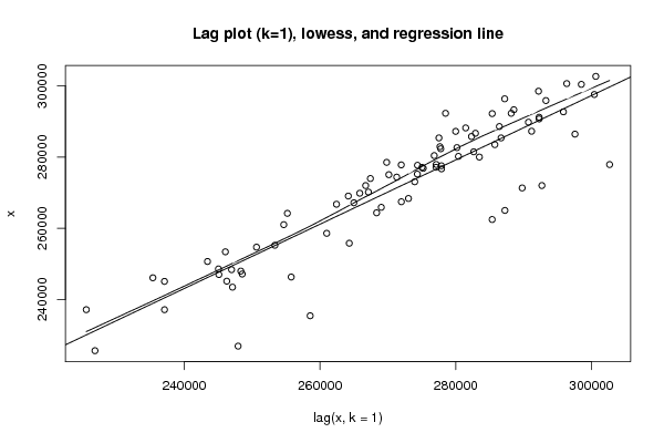
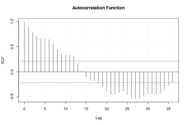
Figures (Output of Computation) | |||||||||||||||||||||||||||||||||||||||||||||||||||||
Input Parameters & R Code | |||||||||||||||||||||||||||||||||||||||||||||||||||||
| Parameters (Session): | |||||||||||||||||||||||||||||||||||||||||||||||||||||
| par1 = 0 ; par2 = 36 ; | |||||||||||||||||||||||||||||||||||||||||||||||||||||
| Parameters (R input): | |||||||||||||||||||||||||||||||||||||||||||||||||||||
| par1 = 0 ; par2 = 36 ; | |||||||||||||||||||||||||||||||||||||||||||||||||||||
| R code (references can be found in the software module): | |||||||||||||||||||||||||||||||||||||||||||||||||||||
par1 <- as.numeric(par1) | |||||||||||||||||||||||||||||||||||||||||||||||||||||