Repository of Reproducible Computations

Free Statistics

of Irreproducible Research!

Author's title

Author

*The author of this computation has been verified*

R Software Module

rwasp_autocorrelation.wasp

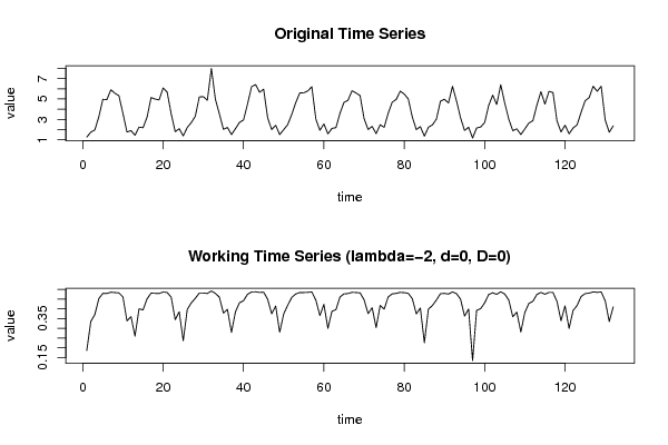
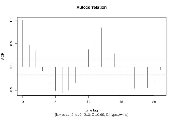
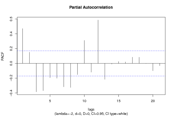
Title produced by software

(Partial) Autocorrelation Function

Date of computation

Wed, 14 Dec 2011 10:45:27 -0500

Cite this page as follows

Statistical Computations at FreeStatistics.org, Office for Research Development and Education, URL https://freestatistics.org/blog/index.php?v=date/2011/Dec/14/t1323877855qgicxb4roxczs9u.htm/, Retrieved Wed, 01 May 2024 22:23:40 +0000

Statistical Computations at FreeStatistics.org, Office for Research Development and Education, URL https://freestatistics.org/blog/index.php?pk=155079, Retrieved Wed, 01 May 2024 22:23:40 +0000

QR Codes:

Paste this QR Code to cite your computation.

Original text written by user:

IsPrivate?

No (this computation is public)

User-defined keywords

Estimated Impact

151

Family? (F = Feedback message, R = changed R code, M = changed R Module, P = changed Parameters, D = changed Data)

-     [Univariate Data Series] [] [2008-12-08 19:22:39] [d2d412c7f4d35ffbf5ee5ee89db327d4]
- RMP   [Spectral Analysis] [] [2011-12-06 19:48:28] [b98453cac15ba1066b407e146608df68]
- R PD    [Spectral Analysis] [] [2011-12-14 15:31:08] [c53df38315e3cbde2dbe0de809195ef2]
- RMP         [(Partial) Autocorrelation Function] [] [2011-12-14 15:45:27] [ff205c8f94ca61ac7cf7eb30cad83105] [Current]
- R P           [(Partial) Autocorrelation Function] [] [2011-12-14 15:52:43] [c53df38315e3cbde2dbe0de809195ef2] 
- RMP           [Variance Reduction Matrix] [] [2011-12-14 15:54:54] [c53df38315e3cbde2dbe0de809195ef2] 
- RMP           [ARIMA Backward Selection] [] [2011-12-14 16:01:54] [c53df38315e3cbde2dbe0de809195ef2] 
- RMPD            [Box-Cox Linearity Plot] [] [2011-12-14 21:42:54] [c53df38315e3cbde2dbe0de809195ef2] 
-    D              [Box-Cox Linearity Plot] [] [2011-12-21 22:01:26] [80bca13c5f9401fbb753952fd2952f4a] 

Feedback Forum

Post a new message

Dataseries X:

Download CSV

Histogram

Boxplots

Summary of computational transaction
Raw Input	view raw input (R code)
Raw Output	view raw output of R engine
Computing time	1 seconds
R Server	'Herman Ole Andreas Wold' @ wold.wessa.net

\begin{tabular}{lllllllll}
\hline
Summary of computational transaction \tabularnewline
Raw Input & view raw input (R code)  \tabularnewline
Raw Output & view raw output of R engine  \tabularnewline
Computing time & 1 seconds \tabularnewline
R Server & 'Herman Ole Andreas Wold' @ wold.wessa.net \tabularnewline
\hline
\end{tabular}
%Source: https://freestatistics.org/blog/index.php?pk=155079&T=0

[TABLE]
[ROW][C]Summary of computational transaction[/C][/ROW]
[ROW][C]Raw Input[/C][C]view raw input (R code) [/C][/ROW]
[ROW][C]Raw Output[/C][C]view raw output of R engine [/C][/ROW]
[ROW][C]Computing time[/C][C]1 seconds[/C][/ROW]
[ROW][C]R Server[/C][C]'Herman Ole Andreas Wold' @ wold.wessa.net[/C][/ROW]
[/TABLE]
Source: https://freestatistics.org/blog/index.php?pk=155079&T=0

Globally Unique Identifier (entire table): ba.freestatistics.org/blog/index.php?pk=155079&T=0

As an alternative you can also use a QR Code:

The GUIDs for individual cells are displayed in the table below:

Summary of computational transaction
Raw Input	view raw input (R code)
Raw Output	view raw output of R engine
Computing time	1 seconds
R Server	'Herman Ole Andreas Wold' @ wold.wessa.net

Autocorrelation Function
Time lag k	ACF(k)	T-STAT	P-value
1	0.470451	5.4051	0
2	0.339125	3.8962	7.7e-05
3	-0.085718	-0.9848	0.163257
4	-0.355495	-4.0843	3.8e-05
5	-0.503509	-5.7849	0
6	-0.548684	-6.3039	0
7	-0.501048	-5.7566	0
8	-0.341605	-3.9247	7e-05
9	-0.059089	-0.6789	0.2492
10	0.371511	4.2683	1.9e-05
11	0.433686	4.9827	1e-06
12	0.838709	9.636	0
13	0.406626	4.6718	4e-06
14	0.285108	3.2756	0.000673
15	-0.083717	-0.9618	0.168945
16	-0.32711	-3.7582	0.000128
17	-0.458487	-5.2676	0
18	-0.49698	-5.7099	0
19	-0.450434	-5.1751	0
20	-0.313259	-3.5991	0.000225
21	-0.058391	-0.6709	0.251739

\begin{tabular}{lllllllll}
\hline
Autocorrelation Function \tabularnewline
Time lag k & ACF(k) & T-STAT & P-value \tabularnewline
1 & 0.470451 & 5.4051 & 0 \tabularnewline
2 & 0.339125 & 3.8962 & 7.7e-05 \tabularnewline
3 & -0.085718 & -0.9848 & 0.163257 \tabularnewline
4 & -0.355495 & -4.0843 & 3.8e-05 \tabularnewline
5 & -0.503509 & -5.7849 & 0 \tabularnewline
6 & -0.548684 & -6.3039 & 0 \tabularnewline
7 & -0.501048 & -5.7566 & 0 \tabularnewline
8 & -0.341605 & -3.9247 & 7e-05 \tabularnewline
9 & -0.059089 & -0.6789 & 0.2492 \tabularnewline
10 & 0.371511 & 4.2683 & 1.9e-05 \tabularnewline
11 & 0.433686 & 4.9827 & 1e-06 \tabularnewline
12 & 0.838709 & 9.636 & 0 \tabularnewline
13 & 0.406626 & 4.6718 & 4e-06 \tabularnewline
14 & 0.285108 & 3.2756 & 0.000673 \tabularnewline
15 & -0.083717 & -0.9618 & 0.168945 \tabularnewline
16 & -0.32711 & -3.7582 & 0.000128 \tabularnewline
17 & -0.458487 & -5.2676 & 0 \tabularnewline
18 & -0.49698 & -5.7099 & 0 \tabularnewline
19 & -0.450434 & -5.1751 & 0 \tabularnewline
20 & -0.313259 & -3.5991 & 0.000225 \tabularnewline
21 & -0.058391 & -0.6709 & 0.251739 \tabularnewline
\hline
\end{tabular}
%Source: https://freestatistics.org/blog/index.php?pk=155079&T=1

[TABLE]
[ROW][C]Autocorrelation Function[/C][/ROW]
[ROW][C]Time lag k[/C][C]ACF(k)[/C][C]T-STAT[/C][C]P-value[/C][/ROW]
[ROW][C]1[/C][C]0.470451[/C][C]5.4051[/C][C]0[/C][/ROW]
[ROW][C]2[/C][C]0.339125[/C][C]3.8962[/C][C]7.7e-05[/C][/ROW]
[ROW][C]3[/C][C]-0.085718[/C][C]-0.9848[/C][C]0.163257[/C][/ROW]
[ROW][C]4[/C][C]-0.355495[/C][C]-4.0843[/C][C]3.8e-05[/C][/ROW]
[ROW][C]5[/C][C]-0.503509[/C][C]-5.7849[/C][C]0[/C][/ROW]
[ROW][C]6[/C][C]-0.548684[/C][C]-6.3039[/C][C]0[/C][/ROW]
[ROW][C]7[/C][C]-0.501048[/C][C]-5.7566[/C][C]0[/C][/ROW]
[ROW][C]8[/C][C]-0.341605[/C][C]-3.9247[/C][C]7e-05[/C][/ROW]
[ROW][C]9[/C][C]-0.059089[/C][C]-0.6789[/C][C]0.2492[/C][/ROW]
[ROW][C]10[/C][C]0.371511[/C][C]4.2683[/C][C]1.9e-05[/C][/ROW]
[ROW][C]11[/C][C]0.433686[/C][C]4.9827[/C][C]1e-06[/C][/ROW]
[ROW][C]12[/C][C]0.838709[/C][C]9.636[/C][C]0[/C][/ROW]
[ROW][C]13[/C][C]0.406626[/C][C]4.6718[/C][C]4e-06[/C][/ROW]
[ROW][C]14[/C][C]0.285108[/C][C]3.2756[/C][C]0.000673[/C][/ROW]
[ROW][C]15[/C][C]-0.083717[/C][C]-0.9618[/C][C]0.168945[/C][/ROW]
[ROW][C]16[/C][C]-0.32711[/C][C]-3.7582[/C][C]0.000128[/C][/ROW]
[ROW][C]17[/C][C]-0.458487[/C][C]-5.2676[/C][C]0[/C][/ROW]
[ROW][C]18[/C][C]-0.49698[/C][C]-5.7099[/C][C]0[/C][/ROW]
[ROW][C]19[/C][C]-0.450434[/C][C]-5.1751[/C][C]0[/C][/ROW]
[ROW][C]20[/C][C]-0.313259[/C][C]-3.5991[/C][C]0.000225[/C][/ROW]
[ROW][C]21[/C][C]-0.058391[/C][C]-0.6709[/C][C]0.251739[/C][/ROW]
[/TABLE]
Source: https://freestatistics.org/blog/index.php?pk=155079&T=1

Globally Unique Identifier (entire table): ba.freestatistics.org/blog/index.php?pk=155079&T=1

As an alternative you can also use a QR Code:

The GUIDs for individual cells are displayed in the table below:

Autocorrelation Function
Time lag k	ACF(k)	T-STAT	P-value
1	0.470451	5.4051	0
2	0.339125	3.8962	7.7e-05
3	-0.085718	-0.9848	0.163257
4	-0.355495	-4.0843	3.8e-05
5	-0.503509	-5.7849	0
6	-0.548684	-6.3039	0
7	-0.501048	-5.7566	0
8	-0.341605	-3.9247	7e-05
9	-0.059089	-0.6789	0.2492
10	0.371511	4.2683	1.9e-05
11	0.433686	4.9827	1e-06
12	0.838709	9.636	0
13	0.406626	4.6718	4e-06
14	0.285108	3.2756	0.000673
15	-0.083717	-0.9618	0.168945
16	-0.32711	-3.7582	0.000128
17	-0.458487	-5.2676	0
18	-0.49698	-5.7099	0
19	-0.450434	-5.1751	0
20	-0.313259	-3.5991	0.000225
21	-0.058391	-0.6709	0.251739

Partial Autocorrelation Function
Time lag k	PACF(k)	T-STAT	P-value
1	0.470451	5.4051	0
2	0.151283	1.7381	0.042262
3	-0.384167	-4.4137	1e-05
4	-0.368318	-4.2317	2.2e-05
5	-0.194526	-2.2349	0.013551
6	-0.200921	-2.3084	0.011265
7	-0.317237	-3.6448	0.000192
8	-0.325934	-3.7447	0.000134
9	-0.151403	-1.7395	0.04214
10	0.31064	3.569	0.00025
11	-0.118778	-1.3647	0.087341
12	0.585911	6.7316	0
13	-0.215949	-2.4811	0.007178
14	-0.009603	-0.1103	0.456156
15	0.02553	0.2933	0.384871
16	0.020284	0.233	0.408042
17	0.084075	0.9659	0.167918
18	0.083408	0.9583	0.169836
19	-0.001749	-0.0201	0.492
20	-0.099912	-1.1479	0.126543
21	-0.030872	-0.3547	0.361692

\begin{tabular}{lllllllll}
\hline
Partial Autocorrelation Function \tabularnewline
Time lag k & PACF(k) & T-STAT & P-value \tabularnewline
1 & 0.470451 & 5.4051 & 0 \tabularnewline
2 & 0.151283 & 1.7381 & 0.042262 \tabularnewline
3 & -0.384167 & -4.4137 & 1e-05 \tabularnewline
4 & -0.368318 & -4.2317 & 2.2e-05 \tabularnewline
5 & -0.194526 & -2.2349 & 0.013551 \tabularnewline
6 & -0.200921 & -2.3084 & 0.011265 \tabularnewline
7 & -0.317237 & -3.6448 & 0.000192 \tabularnewline
8 & -0.325934 & -3.7447 & 0.000134 \tabularnewline
9 & -0.151403 & -1.7395 & 0.04214 \tabularnewline
10 & 0.31064 & 3.569 & 0.00025 \tabularnewline
11 & -0.118778 & -1.3647 & 0.087341 \tabularnewline
12 & 0.585911 & 6.7316 & 0 \tabularnewline
13 & -0.215949 & -2.4811 & 0.007178 \tabularnewline
14 & -0.009603 & -0.1103 & 0.456156 \tabularnewline
15 & 0.02553 & 0.2933 & 0.384871 \tabularnewline
16 & 0.020284 & 0.233 & 0.408042 \tabularnewline
17 & 0.084075 & 0.9659 & 0.167918 \tabularnewline
18 & 0.083408 & 0.9583 & 0.169836 \tabularnewline
19 & -0.001749 & -0.0201 & 0.492 \tabularnewline
20 & -0.099912 & -1.1479 & 0.126543 \tabularnewline
21 & -0.030872 & -0.3547 & 0.361692 \tabularnewline
\hline
\end{tabular}
%Source: https://freestatistics.org/blog/index.php?pk=155079&T=2

[TABLE]
[ROW][C]Partial Autocorrelation Function[/C][/ROW]
[ROW][C]Time lag k[/C][C]PACF(k)[/C][C]T-STAT[/C][C]P-value[/C][/ROW]
[ROW][C]1[/C][C]0.470451[/C][C]5.4051[/C][C]0[/C][/ROW]
[ROW][C]2[/C][C]0.151283[/C][C]1.7381[/C][C]0.042262[/C][/ROW]
[ROW][C]3[/C][C]-0.384167[/C][C]-4.4137[/C][C]1e-05[/C][/ROW]
[ROW][C]4[/C][C]-0.368318[/C][C]-4.2317[/C][C]2.2e-05[/C][/ROW]
[ROW][C]5[/C][C]-0.194526[/C][C]-2.2349[/C][C]0.013551[/C][/ROW]
[ROW][C]6[/C][C]-0.200921[/C][C]-2.3084[/C][C]0.011265[/C][/ROW]
[ROW][C]7[/C][C]-0.317237[/C][C]-3.6448[/C][C]0.000192[/C][/ROW]
[ROW][C]8[/C][C]-0.325934[/C][C]-3.7447[/C][C]0.000134[/C][/ROW]
[ROW][C]9[/C][C]-0.151403[/C][C]-1.7395[/C][C]0.04214[/C][/ROW]
[ROW][C]10[/C][C]0.31064[/C][C]3.569[/C][C]0.00025[/C][/ROW]
[ROW][C]11[/C][C]-0.118778[/C][C]-1.3647[/C][C]0.087341[/C][/ROW]
[ROW][C]12[/C][C]0.585911[/C][C]6.7316[/C][C]0[/C][/ROW]
[ROW][C]13[/C][C]-0.215949[/C][C]-2.4811[/C][C]0.007178[/C][/ROW]
[ROW][C]14[/C][C]-0.009603[/C][C]-0.1103[/C][C]0.456156[/C][/ROW]
[ROW][C]15[/C][C]0.02553[/C][C]0.2933[/C][C]0.384871[/C][/ROW]
[ROW][C]16[/C][C]0.020284[/C][C]0.233[/C][C]0.408042[/C][/ROW]
[ROW][C]17[/C][C]0.084075[/C][C]0.9659[/C][C]0.167918[/C][/ROW]
[ROW][C]18[/C][C]0.083408[/C][C]0.9583[/C][C]0.169836[/C][/ROW]
[ROW][C]19[/C][C]-0.001749[/C][C]-0.0201[/C][C]0.492[/C][/ROW]
[ROW][C]20[/C][C]-0.099912[/C][C]-1.1479[/C][C]0.126543[/C][/ROW]
[ROW][C]21[/C][C]-0.030872[/C][C]-0.3547[/C][C]0.361692[/C][/ROW]
[/TABLE]
Source: https://freestatistics.org/blog/index.php?pk=155079&T=2

Globally Unique Identifier (entire table): ba.freestatistics.org/blog/index.php?pk=155079&T=2

As an alternative you can also use a QR Code:

The GUIDs for individual cells are displayed in the table below:

Partial Autocorrelation Function
Time lag k	PACF(k)	T-STAT	P-value
1	0.470451	5.4051	0
2	0.151283	1.7381	0.042262
3	-0.384167	-4.4137	1e-05
4	-0.368318	-4.2317	2.2e-05
5	-0.194526	-2.2349	0.013551
6	-0.200921	-2.3084	0.011265
7	-0.317237	-3.6448	0.000192
8	-0.325934	-3.7447	0.000134
9	-0.151403	-1.7395	0.04214
10	0.31064	3.569	0.00025
11	-0.118778	-1.3647	0.087341
12	0.585911	6.7316	0
13	-0.215949	-2.4811	0.007178
14	-0.009603	-0.1103	0.456156
15	0.02553	0.2933	0.384871
16	0.020284	0.233	0.408042
17	0.084075	0.9659	0.167918
18	0.083408	0.9583	0.169836
19	-0.001749	-0.0201	0.492
20	-0.099912	-1.1479	0.126543
21	-0.030872	-0.3547	0.361692

Figure 1

PNG link

Postscript link

PDF link

Figure 2

PNG link

Postscript link

PDF link

Figure 3

PNG link

Postscript link

PDF link

Parameters (Session):

par1 = Default ; par2 = -2.0 ; par3 = 0 ; par4 = 0 ; par5 = 12 ; par6 = White Noise ; par7 = 0.95 ;

Parameters (R input):

par1 = Default ; par2 = -2.0 ; par3 = 0 ; par4 = 0 ; par5 = 12 ; par6 = White Noise ; par7 = 0.95 ; par8 = ;

R code (references can be found in the software module):

if (par1 == 'Default') {
par1 = 10*log10(length(x))
} else {
par1 <- as.numeric(par1)
}
par2 <- as.numeric(par2)
par3 <- as.numeric(par3)
par4 <- as.numeric(par4)
par5 <- as.numeric(par5)
if (par6 == 'White Noise') par6 <- 'white' else par6 <- 'ma'
par7 <- as.numeric(par7)
if (par8 != '') par8 <- as.numeric(par8)
ox <- x
if (par8 == '') {
if (par2 == 0) {
x <- log(x)
} else {
x <- (x ^ par2 - 1) / par2
}
} else {
x <- log(x,base=par8)
}
if (par3 > 0) x <- diff(x,lag=1,difference=par3)
if (par4 > 0) x <- diff(x,lag=par5,difference=par4)
bitmap(file='picts.png')
op <- par(mfrow=c(2,1))
plot(ox,type='l',main='Original Time Series',xlab='time',ylab='value')
if (par8=='') {
mytitle <- paste('Working Time Series (lambda=',par2,', d=',par3,', D=',par4,')',sep='')
mysub <- paste('(lambda=',par2,', d=',par3,', D=',par4,', CI=', par7, ', CI type=',par6,')',sep='')
} else {
mytitle <- paste('Working Time Series (base=',par8,', d=',par3,', D=',par4,')',sep='')
mysub <- paste('(base=',par8,', d=',par3,', D=',par4,', CI=', par7, ', CI type=',par6,')',sep='')
}
plot(x,type='l', main=mytitle,xlab='time',ylab='value')
par(op)
dev.off()
bitmap(file='pic1.png')
racf <- acf(x, par1, main='Autocorrelation', xlab='time lag', ylab='ACF', ci.type=par6, ci=par7, sub=mysub)
dev.off()
bitmap(file='pic2.png')
rpacf <- pacf(x,par1,main='Partial Autocorrelation',xlab='lags',ylab='PACF',sub=mysub)
dev.off()
(myacf <- c(racf$acf))
(mypacf <- c(rpacf$acf))
lengthx <- length(x)
sqrtn <- sqrt(lengthx)
load(file='createtable')
a<-table.start()
a<-table.row.start(a)
a<-table.element(a,'Autocorrelation Function',4,TRUE)
a<-table.row.end(a)
a<-table.row.start(a)
a<-table.element(a,'Time lag k',header=TRUE)
a<-table.element(a,hyperlink('basics.htm','ACF(k)','click here for more information about the Autocorrelation Function'),header=TRUE)
a<-table.element(a,'T-STAT',header=TRUE)
a<-table.element(a,'P-value',header=TRUE)
a<-table.row.end(a)
for (i in 2:(par1+1)) {
a<-table.row.start(a)
a<-table.element(a,i-1,header=TRUE)
a<-table.element(a,round(myacf[i],6))
mytstat <- myacf[i]*sqrtn
a<-table.element(a,round(mytstat,4))
a<-table.element(a,round(1-pt(abs(mytstat),lengthx),6))
a<-table.row.end(a)
}
a<-table.end(a)
table.save(a,file='mytable.tab')
a<-table.start()
a<-table.row.start(a)
a<-table.element(a,'Partial Autocorrelation Function',4,TRUE)
a<-table.row.end(a)
a<-table.row.start(a)
a<-table.element(a,'Time lag k',header=TRUE)
a<-table.element(a,hyperlink('basics.htm','PACF(k)','click here for more information about the Partial Autocorrelation Function'),header=TRUE)
a<-table.element(a,'T-STAT',header=TRUE)
a<-table.element(a,'P-value',header=TRUE)
a<-table.row.end(a)
for (i in 1:par1) {
a<-table.row.start(a)
a<-table.element(a,i,header=TRUE)
a<-table.element(a,round(mypacf[i],6))
mytstat <- mypacf[i]*sqrtn
a<-table.element(a,round(mytstat,4))
a<-table.element(a,round(1-pt(abs(mytstat),lengthx),6))
a<-table.row.end(a)
}
a<-table.end(a)
table.save(a,file='mytable1.tab')

Free Statistics

Description of Statistical Computation

Tree of Dependent Computations

Dataset

Tables (Output of Computation)

Figures (Output of Computation)

Input Parameters & R Code