Repository of Reproducible Computations

Free Statistics

of Irreproducible Research!

Author's title

Author

*The author of this computation has been verified*

R Software Module

rwasp_density.wasp

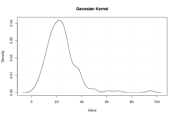
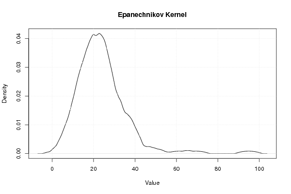
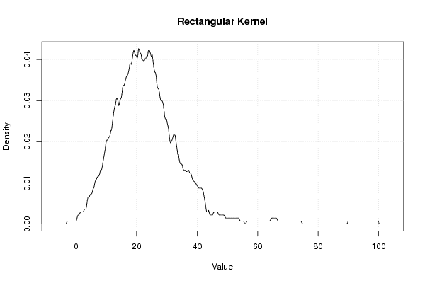
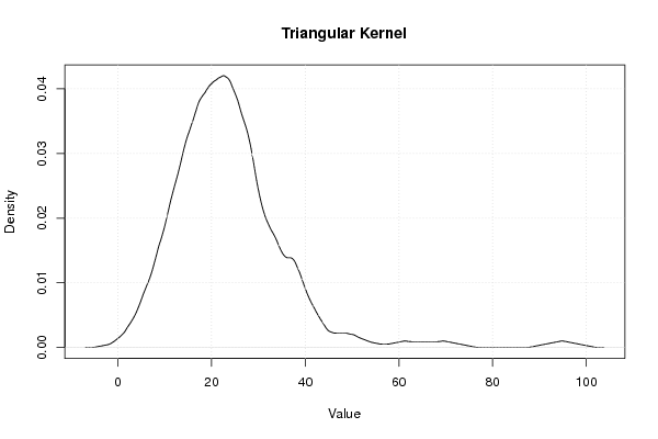
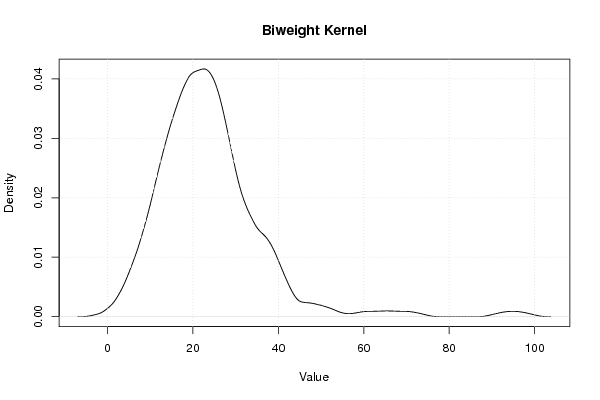
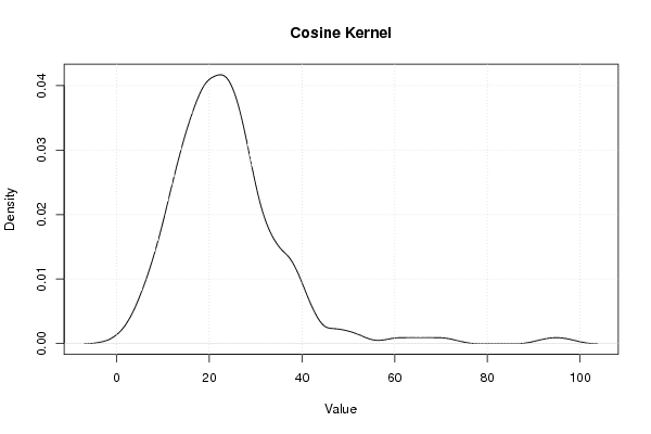
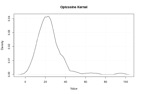
Title produced by software

Kernel Density Estimation

Date of computation

Tue, 13 Dec 2011 09:43:33 -0500

Cite this page as follows

Statistical Computations at FreeStatistics.org, Office for Research Development and Education, URL https://freestatistics.org/blog/index.php?v=date/2011/Dec/13/t1323787438gqwf2l6xm0t8agk.htm/, Retrieved Thu, 02 May 2024 17:40:13 +0000

Statistical Computations at FreeStatistics.org, Office for Research Development and Education, URL https://freestatistics.org/blog/index.php?pk=154405, Retrieved Thu, 02 May 2024 17:40:13 +0000

QR Codes:

Paste this QR Code to cite your computation.

Original text written by user:

IsPrivate?

No (this computation is public)

User-defined keywords

Estimated Impact

128

Family? (F = Feedback message, R = changed R code, M = changed R Module, P = changed Parameters, D = changed Data)

-     [Recursive Partitioning (Regression Trees)] [] [2010-12-05 20:30:15] [b98453cac15ba1066b407e146608df68]
- RMPD    [Kernel Density Estimation] [] [2011-12-13 14:43:33] [885a9dbaf162325773a0a0afdf9f947e] [Current]
- RMPD      [Central Tendency] [] [2011-12-13 14:58:14] [c4580079d5d2b3f0ba412f27cdc441be] 
-    D      [Kernel Density Estimation] [] [2011-12-13 15:00:16] [c4580079d5d2b3f0ba412f27cdc441be] 
- RM D      [Histogram] [] [2011-12-13 15:44:18] [c4580079d5d2b3f0ba412f27cdc441be] 
- RM D      [Harrell-Davis Quantiles] [] [2011-12-13 15:50:11] [c4580079d5d2b3f0ba412f27cdc441be] 
- RM D      [Harrell-Davis Quantiles] [] [2011-12-13 16:08:07] [c4580079d5d2b3f0ba412f27cdc441be] 

Feedback Forum

Post a new message

Dataseries X:

Download CSV

Histogram

Boxplots

28.23472222
28.05861111
1.993333333
26.82222222
48.84
94.88055556
28.77694444
31.28083333
23.77055556
61.33361111
25.73916667
37.03555556
17.04472222
34.98055556
22.86555556
28.33611111
28.20083333
11.54611111
27.75638889
6.291111111
12.97166667
36.58277778
25.48194444
22.18416667
30.01194444
27.46277778
33.45694444
32.23555556
69.4575
37.80111111
25.69416667
37.71694444
20.66888889
22.56666667
37.04666667
27.26277778
22.11638889
16.44277778
38.87277778
32.94777778
20.24444444
18.1875
27.67861111
19.99027778
21.46444444
13.69138889
37.53638889
30.12388889
24.92944444
12.30444444
21.56888889
50.42444444
37.2275
34.46222222
25.73055556
33.84666667
14.69861111
22.74222222
16.38361111
14.86527778
16.89222222
15.65972222
18.19166667
22.48583333
21.195
28.89194444
27.25111111
18.88583333
8.608055556
37.62722222
20.41777778
17.53416667
17.015
20.80944444
8.826111111
22.62138889
24.21833333
13.91388889
18.2625
15.73694444
43.99972222
12.90416667
20.45111111
10.66527778
25.5275
38.75722222
14.49
14.32416667
19.5975
23.57111111
28.48277778
24.07722222
23.80805556
9.628333333
41.82777778
27.66972222
5.374722222
27.60361111
23.95277778
8.565833333
8.807222222
24.94611111
17.24666667
11.15305556
7.676111111
21.38611111
10.40555556
15.04361111
13.85055556
23.42694444
17.82638889
16.495
33.14111111
21.30611111
28.72916667
19.54
12.05833333
29.12166667
17.28194444
19.25111111
14.75472222
5.49
24.07777778
23.3625
21.65138889
24.75361111
25.27916667
11.18
17.82972222
14.12694444
15.72583333
17.44222222
20.14861111

Summary of computational transaction
Raw Input	view raw input (R code)
Raw Output	view raw output of R engine
Computing time	3 seconds
R Server	'Herman Ole Andreas Wold' @ wold.wessa.net

\begin{tabular}{lllllllll}
\hline
Summary of computational transaction \tabularnewline
Raw Input & view raw input (R code)  \tabularnewline
Raw Output & view raw output of R engine  \tabularnewline
Computing time & 3 seconds \tabularnewline
R Server & 'Herman Ole Andreas Wold' @ wold.wessa.net \tabularnewline
\hline
\end{tabular}
%Source: https://freestatistics.org/blog/index.php?pk=154405&T=0

[TABLE]
[ROW][C]Summary of computational transaction[/C][/ROW]
[ROW][C]Raw Input[/C][C]view raw input (R code) [/C][/ROW]
[ROW][C]Raw Output[/C][C]view raw output of R engine [/C][/ROW]
[ROW][C]Computing time[/C][C]3 seconds[/C][/ROW]
[ROW][C]R Server[/C][C]'Herman Ole Andreas Wold' @ wold.wessa.net[/C][/ROW]
[/TABLE]
Source: https://freestatistics.org/blog/index.php?pk=154405&T=0

Globally Unique Identifier (entire table): ba.freestatistics.org/blog/index.php?pk=154405&T=0

As an alternative you can also use a QR Code:

The GUIDs for individual cells are displayed in the table below:

Summary of computational transaction
Raw Input	view raw input (R code)
Raw Output	view raw output of R engine
Computing time	3 seconds
R Server	'Herman Ole Andreas Wold' @ wold.wessa.net

Properties of Density Trace
Bandwidth	2.97819278480695
#Observations	133

\begin{tabular}{lllllllll}
\hline
Properties of Density Trace \tabularnewline
Bandwidth & 2.97819278480695 \tabularnewline
#Observations & 133 \tabularnewline
\hline
\end{tabular}
%Source: https://freestatistics.org/blog/index.php?pk=154405&T=1

[TABLE]
[ROW][C]Properties of Density Trace[/C][/ROW]
[ROW][C]Bandwidth[/C][C]2.97819278480695[/C][/ROW]
[ROW][C]#Observations[/C][C]133[/C][/ROW]
[/TABLE]
Source: https://freestatistics.org/blog/index.php?pk=154405&T=1

Globally Unique Identifier (entire table): ba.freestatistics.org/blog/index.php?pk=154405&T=1

As an alternative you can also use a QR Code:

The GUIDs for individual cells are displayed in the table below:

Properties of Density Trace
Bandwidth	2.97819278480695
#Observations	133

Figure 1

PNG link

Postscript link

PDF link

Figure 2

PNG link

Postscript link

PDF link

Figure 3

PNG link

Postscript link

PDF link

Figure 4

PNG link

Postscript link

PDF link

Figure 5

PNG link

Postscript link

PDF link

Figure 6

PNG link

Postscript link

PDF link

Figure 7

PNG link

Postscript link

PDF link

Parameters (Session):

par1 = 0 ;

Parameters (R input):

par1 = 0 ;

R code (references can be found in the software module):

if (par1 == '0') bw <- 'nrd0'
if (par1 != '0') bw <- as.numeric(par1)
bitmap(file='density1.png')
mydensity1<-density(x,bw=bw,kernel='gaussian',na.rm=TRUE)
plot(mydensity1,main='Gaussian Kernel',xlab=xlab,ylab=ylab)
grid()
dev.off()
mydensity1
bitmap(file='density2.png')
mydensity2<-density(x,bw=bw,kernel='epanechnikov',na.rm=TRUE)
plot(mydensity2,main='Epanechnikov Kernel',xlab=xlab,ylab=ylab)
grid()
dev.off()
bitmap(file='density3.png')
mydensity3<-density(x,bw=bw,kernel='rectangular',na.rm=TRUE)
plot(mydensity3,main='Rectangular Kernel',xlab=xlab,ylab=ylab)
grid()
dev.off()
bitmap(file='density4.png')
mydensity4<-density(x,bw=bw,kernel='triangular',na.rm=TRUE)
plot(mydensity4,main='Triangular Kernel',xlab=xlab,ylab=ylab)
grid()
dev.off()
bitmap(file='density5.png')
mydensity5<-density(x,bw=bw,kernel='biweight',na.rm=TRUE)
plot(mydensity5,main='Biweight Kernel',xlab=xlab,ylab=ylab)
grid()
dev.off()
bitmap(file='density6.png')
mydensity6<-density(x,bw=bw,kernel='cosine',na.rm=TRUE)
plot(mydensity6,main='Cosine Kernel',xlab=xlab,ylab=ylab)
grid()
dev.off()
bitmap(file='density7.png')
mydensity7<-density(x,bw=bw,kernel='optcosine',na.rm=TRUE)
plot(mydensity7,main='Optcosine Kernel',xlab=xlab,ylab=ylab)
grid()
dev.off()
load(file='createtable')
a<-table.start()
a<-table.row.start(a)
a<-table.element(a,'Properties of Density Trace',2,TRUE)
a<-table.row.end(a)
a<-table.row.start(a)
a<-table.element(a,'Bandwidth',header=TRUE)
a<-table.element(a,mydensity1$bw)
a<-table.row.end(a)
a<-table.row.start(a)
a<-table.element(a,'#Observations',header=TRUE)
a<-table.element(a,mydensity1$n)
a<-table.row.end(a)
a<-table.end(a)
table.save(a,file='mytable.tab')

Free Statistics

Description of Statistical Computation

Tree of Dependent Computations

Dataset

Tables (Output of Computation)

Figures (Output of Computation)

Input Parameters & R Code